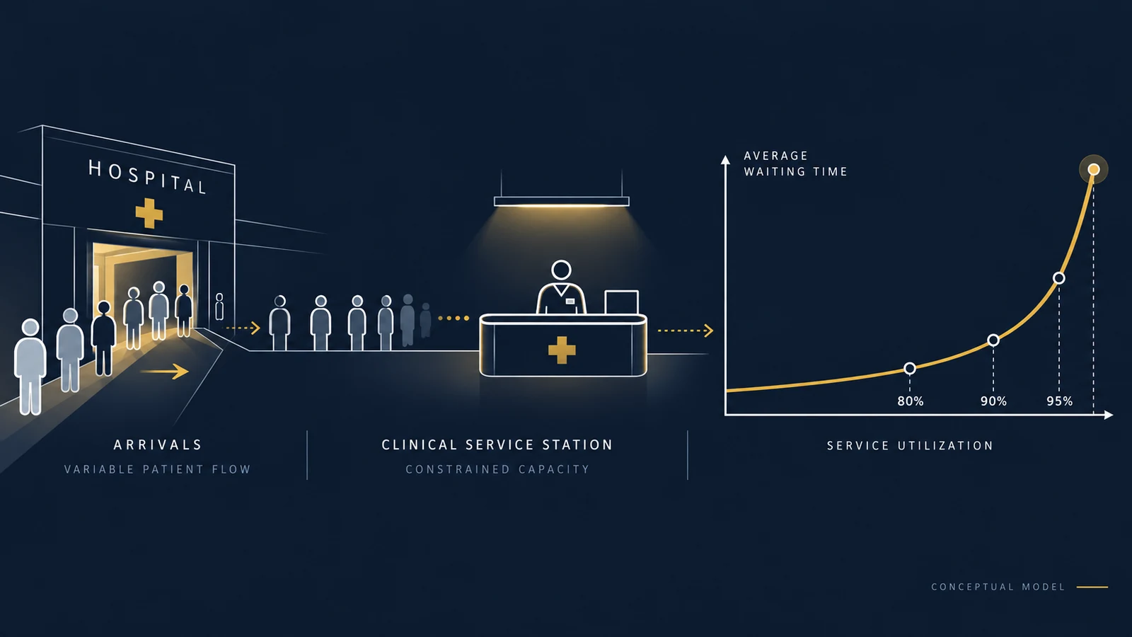
A hospital reports that one of its operational resources is operating at 85% utilization.
On paper, that sounds reasonable.
There is still 15% unused capacity.
Yet patients are waiting longer than expected, clinicians are experiencing delays, and managers are discussing whether additional resources are necessary.
How can a system have unused capacity and still experience substantial waiting?
The answer often involves a fundamental distinction:
Average capacity utilization is not the same as the ability to absorb variable demand without delay.
In systems where arrivals and service times fluctuate, waiting can increase rapidly as utilization approaches capacity.
This is a central insight from queueing theory, a branch of operations research concerned with arrivals, service processes, congestion, and waiting.
For healthcare organizations, the practical question is not simply: “How busy are we?”
It is: “Can our available resources handle the variability in patient demand while maintaining acceptable access, safety, and service times?”
That requires looking beyond average utilization.
Why Waiting Times Can Increase Before Capacity Reaches 100%
Consider a service process with a theoretical maximum capacity of ten patients per hour. If eight patients arrive per hour, average utilization is 8 / 10 = 80%. If nine arrive, it is 90%. If 9.5 arrive, it is 95%.
These values describe average demand relative to average service capacity. They do not tell us how evenly patients arrive or whether service times are consistent.
Patients rarely arrive at perfectly spaced intervals. Some periods are quiet; others experience several arrivals close together. Service requirements also differ: one patient may require a short interaction, while another may require substantially more time.
When arrivals overlap with ongoing service, a queue can form even if average demand remains below average capacity. As utilization increases, the system has less spare capacity available to clear those queues. The result can be a nonlinear increase in waiting time.
A Worked Example Using Queueing Theory
To illustrate the relationship, consider a simplified M/M/1 queue. The model assumes arrivals follow a Poisson process, service times are exponentially distributed, one service station handles patients, service is first-come, first-served, the system has sufficient waiting space, arrival and service rates are stable, and arrivals remain below the service rate.
The notation M/M/1 refers to the stochastic arrival process, stochastic service process, and one server. This is a teaching model, not a representation of a full emergency department. Real hospitals have multiple service stations, patient priorities, shared resources, complex care pathways, and downstream constraints.
Let λ be the average arrival rate and μ the average service rate. Utilization is ρ = λ / μ. For a stable M/M/1 queue, λ < μ. The expected total time in the system is:
W = 1 / (μ − λ)
This includes waiting and service. Expected waiting time before service starts is:
Wq = W − (1 / μ)
These are standard results under the stated assumptions; see the MIT OpenCourseWare M/M/1 queue lecture for an instructional treatment.
What Happens as Utilization Increases?
Assume the service station can process an average of 10 patients per hour, so μ = 10. Average service time is 1 / 10 hour, or 6 minutes per patient.
Scenario A: 80% utilization
λ = 8 patients/hour; ρ = 8 / 10 = 80%.
W = 1 / (10 − 8) = 0.5 hours = 30 minutes
Wq = 30 − 6 = 24 minutes
Scenario B: 90% utilization
λ = 9 patients/hour; ρ = 9 / 10 = 90%.
W = 1 / (10 − 9) = 1 hour = 60 minutes
Wq = 60 − 6 = 54 minutes
Scenario C: 95% utilization
λ = 9.5 patients/hour; ρ = 9.5 / 10 = 95%.
W = 1 / (10 − 9.5) = 2 hours = 120 minutes
Wq = 120 − 6 = 114 minutes
Comparing the three scenarios
| Arrival rate | Utilization | Average queue wait | Average time in system |
|---|---|---|---|
| 8 patients/hour | 80% | 24 minutes | 30 minutes |
| 9 patients/hour | 90% | 54 minutes | 60 minutes |
| 9.5 patients/hour | 95% | 114 minutes | 120 minutes |
All figures come from the same illustrative M/M/1 model. The service rate and average service time remain constant; only the arrival rate changes. Increasing utilization from 80% to 95% moves expected time in the system from 30 to 120 minutes—a fourfold increase. The increase in queue waiting is even more pronounced.
This does not establish that a real hospital operating at 95% utilization will have a two-hour average wait. Actual outcomes depend on arrival patterns, staffing, service-time distributions, patient mix, scheduling, priorities, and resource structure. The example demonstrates a mathematical property of a particular queueing model: variable systems can experience substantial congestion before average utilization reaches 100%.
Why the Last Few Percentage Points Matter
At low utilization, a service station often has idle time. That time may look inefficient, but it provides flexibility. When several patients arrive close together, the system has opportunities to clear the queue.
At higher utilization, the service station spends more time continuously occupied. Temporary queues are less likely to disappear quickly. In the M/M/1 expression W = 1 / (μ − λ), as λ approaches μ the denominator approaches zero and predicted waiting rises sharply.
This explains why utilization and waiting need not have a linear relationship. A five-percentage-point increase in utilization does not imply a five-percentage-point increase in waiting. The impact can be much larger under the model assumptions.
Little's Law Connects Patient Volume, Waiting, and Work in Progress
Little’s Law relates average flow, time, and the number of entities in a stable system:
L = λ × W
Here, L is the average number of patients in the system, λ is the long-run average throughput rate, and W is average time in the system. The relationship applies much more broadly than the M/M/1 model, provided the system is stable and measurement boundaries and time units are consistent.
Using the 95% example, λ = 9.5 patients/hour and W = 2 hours:
L = 9.5 × 2 = 19 patients
Under the illustrative model, the average number in the system is 19, including patients waiting and the patient receiving service. The expected queue alone is:
Lq = λ × Wq = 9.5 × 1.9 = 18.05 patients
These are long-run model expectations, not claims about an actual hospital census. The relationship can help analysts check whether patient-flow metrics are internally consistent. If an organization reports throughput, length of stay, and average census, those quantities should reconcile under matching definitions and periods. Care is needed when demand changes over time, the system is not stable, or measurement boundaries differ.
Hospital Capacity Is Not One Number
Hospitals contain several forms of capacity: physical beds, staffed beds, nursing and physician coverage, imaging, laboratory, operating-room, transport, inpatient admission, and discharge-processing capacity. These resources are not interchangeable.
An emergency department may have an available examination room but no clinician immediately available. A patient may be ready for inpatient admission while no appropriate staffed bed is available. A diagnostic test may be ordered promptly but delayed by laboratory or imaging capacity. A patient may have completed treatment but remain in a bed while waiting for transport or discharge coordination.
Reported occupancy therefore may not describe the capacity of the process constraining patient flow. A more useful question is: Which resource or transition is limiting the movement of patients through the system? That is a bottleneck question.
Emergency Department Crowding Can Be a Hospital-Wide Problem
The Agency for Healthcare Research and Quality guide to identifying patient-flow strategies recommends understanding likely causes of a specific flow problem before selecting an intervention. The Institute for Healthcare Improvement’s hospital-flow program likewise frames flow around coordinated, hospital-wide care, appropriate placement, timely transitions, and available capacity.
These perspectives recognize that emergency department congestion may originate outside the emergency department. An admitted patient who is ready to leave the ED but must wait for an inpatient bed may continue occupying an ED treatment space, limiting capacity for new arrivals.
The Institute for Healthcare Improvement’s discussion of hospital-wide patient flow likewise describes an interconnected system where delays in one unit can affect emergency department waits elsewhere.
Even when ED staff work efficiently, downstream boarding can constrain throughput. An intervention aimed at the wrong stage may have little effect: adding triage staff, for example, may not resolve a problem primarily caused by delayed inpatient bed availability. The right response depends on the actual bottleneck.
A Patient-Flow Timeline Is More Useful Than One Average
Suppose a hospital reports an average ED length of stay of 240 minutes. That summarizes an outcome but does not explain where the time was spent. A stage-level view might look like this:
| Stage | Illustrative duration |
|---|---|
| Arrival to first clinician | 35 minutes |
| Initial assessment and testing | 65 minutes |
| Results and disposition decision | 40 minutes |
| Admission decision to ED departure | 100 minutes |
| Total | 240 minutes |
These durations are hypothetical. The largest segment occurs after the admission decision, suggesting an investigation into inpatient placement and transfer. It does not prove that inpatient capacity is the cause; actual timestamps, bed availability, staffing, acuity, and operating context would need to be examined. Stage-level measurement turns one broad KPI into testable operational questions.
Define the Metrics Before Building the Dashboard
Patient-flow reporting can mislead when definitions differ. Document the events and boundaries used for measures such as:
- Door-to-provider time: arrival to first qualifying clinician contact, with that event explicitly defined.
- ED length of stay: ED arrival to physical departure from the department.
- Boarding time: the defined admission decision or bed-request event to physical ED departure, using a stated convention.
- Staffed capacity: resources operationally available with the necessary staff and support.
- Utilization: observed demand or occupied resource time relative to relevant available capacity over a specified interval.
- Throughput: patients completing a defined process per unit of time.
Organizations may define events differently. Standardize them before comparing departments, facilities, or periods. An apparent improvement can otherwise reflect a measurement change rather than an operational one. A decision-first KPI framework can help connect definitions to decisions and owners.
Why Daily Averages Can Hide the Real Problem
Imagine two departments each receiving an average of 120 patients per day. One has relatively stable arrivals; the other has substantial afternoon and evening peaks. Their daily average volume is identical, but their waiting-time distributions may differ.
Capacity planning based only on daily averages can miss shorter periods when arrivals approach or exceed available service capacity. A more informative analysis may examine arrivals by hour and day of week, acuity mix, staffed capacity by shift, service-time distributions, queue length, and delays at key process transitions.
The measurement interval matters: a daily or monthly average can conceal an operational bottleneck lasting several hours.
Average Waiting Time Is Not Enough
Two hospitals may report the same mean wait of 40 minutes even though one has relatively consistent waits and the other has many short waits plus a meaningful tail of much longer delays. The mean alone does not reveal that difference.
Supplementary measures can include median, 90th- and 95th-percentile waiting times, the percentage exceeding a defined threshold, and waiting time by acuity or arrival period. These help distinguish typical performance from extreme delays. Clinical urgency matters: operational thresholds should be established with clinical leadership and appropriate safety considerations.
What Happens If Capacity Increases?
Return to the simplified M/M/1 example. If λ remains 9.5 patients/hour and μ rises from 10 to 11 patients/hour, expected time in the system changes from 1 / (10 − 9.5) = 2 hours (120 minutes) to:
W = 1 / (11 − 9.5) = 0.6667 hours ≈ 40 minutes
In this illustrative model, a 10% increase in service rate reduces expected system time from 120 to about 40 minutes. This is not a predicted hospital outcome, and it does not mean one additional staff member necessarily increases real capacity by 10%. Effects depend on parallel resources, workflow, patient complexity, handoffs, and downstream bottlenecks. The example demonstrates why targeted changes can have disproportionate modeled effects near congestion.
Adding Capacity Is Not Always the Best Intervention
Managers can investigate demand peaks, shift scheduling, diagnostic turnaround, bed assignment, discharge coordination, transport delays, resource pooling, and process variation. Some interventions increase effective capacity; others reduce variability or shorten the time patients occupy constrained resources.
Improving discharge coordination might make staffed beds available earlier, which could reduce boarding under some conditions. The effect should be evaluated using actual operational data. A theoretical model can identify scenarios worth examining; it cannot substitute for validating the hospital’s real constraints.
When Is a Simple Queueing Model Enough?
A simple analytical model can help explain utilization and congestion, check the plausibility of capacity assumptions, compare stylized scenarios, and identify parameters that deserve closer investigation. But a single-server M/M/1 model may be inadequate when a decision depends on multiple parallel clinicians, acuity-based priorities, patient-specific service requirements, time-varying arrivals, scheduled and unscheduled demand, downstream bed constraints, shared resources, or complex patient pathways.
Those questions may call for multi-server or time-varying queueing models, or discrete-event simulation that represents individual patients moving through events and competing for constrained resources: arrival, triage, assessment, diagnostics, treatment, admission decision, bed assignment, and departure.
The appropriate method depends on the decision and available data. A more complicated model is not automatically better; use only the complexity needed to answer the operational question credibly. For decisions involving uncertainty across several plausible futures, see scenario analysis and Monte Carlo simulation.
A Practical Hospital Capacity Analysis
1. Define the decision
Examples include whether to introduce additional clinical coverage during peak hours, whether faster inpatient bed assignment could reduce boarding, which resource constrains throughput, or what capacity is needed to meet a clinically appropriate waiting-time target. The decision determines the model.
2. Reconstruct patient flow
Use operational timestamps to reconstruct events such as arrival, triage, first clinician contact, test order and result, disposition decision, bed request and assignment, and physical departure. Relevant data may also include encounter identifiers, acuity, and service category. Apply appropriate data governance and de-identification; protected health information does not belong in public reporting or examples.
3. Measure demand and available capacity
Estimate arrivals by interval, service completion rates, staffed resources, availability, patient mix, and process-time distributions. Use consistent units and definitions.
4. Identify the constraint
Determine whether dominant delay occurs before assessment, during diagnostics or treatment, or after the disposition decision. Investigate whether the constraint changes across shifts or patient groups.
5. Compare operational scenarios
Evaluate plausible staffing schedules, earlier discharge coordination, bed-assignment workflows, diagnostic turnaround, or resource allocation. Compare waits, throughput, utilization, cost, safety measures, and uncertainty. The goal is not simply to minimize average waiting time; it is to find feasible improvements that support safe, timely, and efficient care.
A Decision-Oriented Capacity Scorecard
| Dimension | Example measure | Decision supported |
|---|---|---|
| Demand | Arrivals by hour | Match resources to peak periods |
| Capacity | Staffed resources by shift | Identify capacity gaps |
| Congestion | Queue length and wait percentiles | Detect excessive delays |
| Throughput | Completed encounters per hour | Evaluate process performance |
| Boarding | Decision-to-departure time | Investigate downstream constraints |
| Reliability | Share within defined time targets | Monitor service consistency |
| Safety | Clinically relevant balancing measures | Avoid unsafe optimization |
Measures should not be interpreted independently. Higher throughput is not necessarily an improvement if clinical outcomes or workload safety deteriorate. Operational analytics should connect efficiency with quality and safety.
Does Reducing Utilization Cause Better Outcomes?
Queueing models demonstrate mathematical relationships under specified assumptions. Observed hospital data are more complicated. If utilization falls and waits shorten, the observation alone does not prove lower utilization caused the improvement; patient volume, case mix, staffing, diagnostics, or inpatient bed availability may also have changed.
Likewise, an association between boarding time and outcomes does not by itself establish the causal effect of boarding. Evaluation requires an appropriate design and attention to confounding and other sources of bias. Prospective evaluations, controlled comparisons, interrupted time-series approaches, or other suitable designs may help where feasible.
A queueing model describes a defined system under its assumptions. An observational analysis describes relationships in recorded data. A causal evaluation asks what changed because of an intervention. These are related but distinct analytical tasks.
What Should Hospital Leadership Take Away?
The central mistake is treating unused average capacity as proof that a system should not experience delays. In variable systems, spare capacity has operational value: it helps absorb unexpected arrivals and fluctuations in service requirements. As utilization approaches effective capacity, waiting can increase disproportionately.
No single utilization percentage is universally appropriate for every hospital, department, or resource. The acceptable operating range depends on variability, patient acuity, resource flexibility, clinical urgency, available alternatives, and the consequences of delay.
Define the care pathway → Measure arrivals and capacity → Identify bottlenecks → Quantify delays → Model alternatives → Validate operational outcomes.
The goal is not to maximize utilization at all costs. It is to design a system capable of delivering appropriate care, in the right place, at the right time, with acceptable safety and operational performance.
References / Further Reading
- MIT OpenCourseWare — M/M/1 Queue, Introduction to Manufacturing Systems
- Agency for Healthcare Research and Quality — Improving Patient Flow and Reducing Emergency Department Crowding, Section 4: Identifying Strategies
- Institute for Healthcare Improvement — Hospital Flow Professional Development Program
- Institute for Healthcare Improvement — Guiding the Flock: 3 Simple Rules to Improve Hospital-wide Patient Flow
Improve Healthcare Decisions With Better Operational Analytics
UAD Consulting supports healthcare analytics, operational measurement, and decision modeling to help organizations understand bottlenecks, evaluate uncertainty, and compare potential improvements using reliable data.
Explore ServicesGet in Touch