A customer support manager reviews the company's weekly performance dashboard.
The team receives approximately 48 calls per hour.
Each call requires five minutes of an agent's time.
Management calculates:
Since one agent provides 60 minutes of capacity per hour, the company needs:
The calculation appears straightforward.
But when the company schedules five agents, customers still experience long waiting times.
Even six agents struggle to meet the organization's response-time target.
Why?
Because customer requests do not arrive at perfectly regular intervals.
Some minutes are quiet.
Other minutes bring several calls simultaneously.
An agent may be available on average while every agent is busy at the exact moment another customer calls.
This is why staffing decisions require more than dividing total workload by employee capacity.
The missing concept is queueing.
The Short Answer: Average Workload Is Not Enough
A useful support staffing model considers five important quantities:
- The number of customer requests arriving.
- The time required to handle each request.
- The number of agents simultaneously available.
- The maximum acceptable waiting time.
- The percentage of customers who should receive service within that time.
A business might establish a target such as:
"At least 80% of incoming calls should be answered within 30 seconds."
This is a service-level requirement.
It is different from average employee utilization.
A team can operate below full utilization and still miss its response-time target.
Queueing theory helps explain why.
One commonly used analytical approach is the Erlang C model.
Under its assumptions, Erlang C estimates the probability that an arriving customer must wait because every agent is busy.
That probability can then be translated into expected response-time performance.
However, the result is a model estimate, not a guarantee of actual performance.
Why Does Average Capacity Underestimate Staffing Needs?
Return to the hypothetical support operation.
The company receives 48 calls per hour.
Average handling time is five minutes.
Total expected workload is:
That equals four agent-hours of work.
This quantity is called offered load.
In queueing theory, offered load is often expressed in Erlangs.
One Erlang represents enough average workload to occupy one server continuously.
Therefore:
Offered load = 4 Erlangs.
Does that mean four agents are sufficient?
No.
Four agents would have exactly enough capacity to handle the expected workload if every minute could be used perfectly.
But arrivals and service durations vary.
Under the standard Erlang C assumptions, a system with four Erlangs of offered load and four agents has utilization of 100%.
It does not have a stable steady-state queue.
Even small periods of excess demand can create backlogs that take time to clear.
Adding a fifth agent creates spare capacity.
But whether that spare capacity is sufficient depends on the response-time requirement.
What Is the Erlang C Queueing Model?
Erlang C is associated with the M/M/c queueing model.
The notation describes a system with:
- Random arrivals following a Poisson process.
- Exponentially distributed service times.
- A fixed number of parallel servers.
- A shared waiting queue.
The model also assumes that customers do not abandon the queue while waiting.
For a conventional application, agents are treated as statistically equivalent servers handling one customer at a time.
The model describes steady-state performance under constant parameters.
These assumptions simplify the problem.
Real support operations may violate them.
Nevertheless, Erlang C provides a useful analytical starting point for understanding how staffing levels affect waiting times.
The four essential inputs
The model requires:
Arrival rate
How many requests arrive during a specified period?
Average handling time
How long does an agent spend handling each request?
For telephone support, this may include talk time, hold time, and after-call work.
Number of available agents
How many agents can actively handle requests during the period?
Response-time target
How quickly should customers receive service?
For example:
80% of calls answered within 30 seconds.
The first three inputs determine the queue's operating characteristics.
The response-time target helps determine whether the resulting staffing level is acceptable.
A Worked Example: Five, Six, Seven, or Eight Agents?
Consider a hypothetical customer support operation.
Assume:
| Input | Value |
|---|---|
| Incoming calls | 48 per hour |
| Average handling time | 5 minutes |
| Offered load | 4 Erlangs |
| Response-time target | 30 seconds |
| Required service level | 80% |
| Available agents | 5 to 8 |
Assume the operation follows the standard Erlang C model.
The calculations below are theoretical model outputs, not observations from an actual support center.
Step 1: Calculate offered load
The offered load is:
A = Arrival rate × Average handling time
Both inputs must use compatible units.
Using hours:
A = 48 × (5 / 60)
A = 4 Erlangs.
This means the incoming workload requires an average of four simultaneously busy agents.
It does not determine the appropriate staffing level by itself.
Step 2: Calculate agent utilization
Under the model:
Utilization = Offered load / Available agents
For five agents:
For six agents:
For seven agents:
For eight agents:
Notice that utilization declines as staffing increases.
But utilization alone does not tell us how long customers will wait.
Step 3: Estimate waiting probability
The Erlang C formula calculates the probability that an arriving customer finds all agents busy.
For offered load A and c agents:
P(wait) = B / (D + B)
where:
B = (A^c / c!) × c / (c - A)
and:
D = sum of A^k / k!
for k = 0 through c - 1.
This formula applies to the stable M/M/c model when c > A.
The waiting probability can then be used to calculate service level.
For a target waiting time t:
Service level(t)
=
1 - P(wait) × exp[-(c - A) × t / AHT]
The waiting-time target and average handling time must use the same time units.
Step 4: Compare staffing scenarios
Using the stated assumptions:
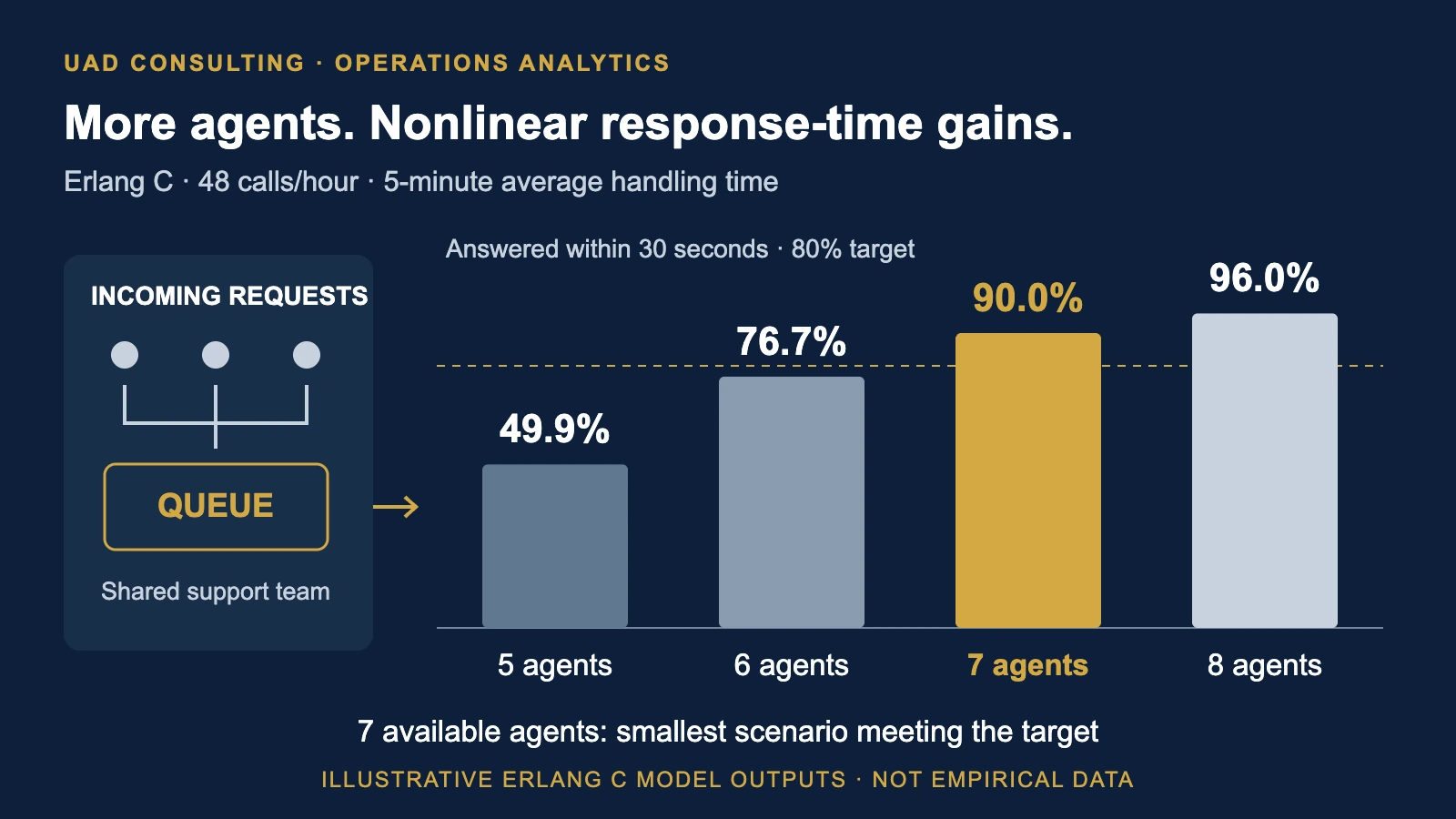
| Agents | Utilization | Probability of Waiting | Answered Within 30 Seconds |
|---|---|---|---|
| 5 | 80.0% | 55.4% | 49.9% |
| 6 | 66.7% | 28.5% | 76.7% |
| 7 | 57.1% | 13.5% | 90.0% |
| 8 | 50.0% | 5.9% | 96.0% |
These values are rounded Erlang C model calculations.
They assume the arrival rate and service-time distribution remain constant.
The results are revealing.
With five agents, the team has 20% spare capacity on average.
Yet only approximately 49.9% of calls are predicted to be answered within 30 seconds.
With six agents, utilization falls to approximately 66.7%.
But the modeled service level is still only 76.7%.
That misses the 80% target.
With seven agents, the predicted service level increases to 90.0%.
Therefore, under the stated assumptions, seven available agents are the smallest staffing level among these scenarios that meets the service-level target.
Eight agents would improve the modeled response time further.
But management must decide whether that additional improvement justifies the cost.
Why Does One Additional Agent Make Such a Large Difference?
Compare six and seven agents.
Six agents:
76.7% answered within 30 seconds.
Seven agents:
90.0% answered within 30 seconds.
The difference is approximately:
= 13.3 percentage points.
At 48 incoming calls per hour, the modeled difference corresponds to approximately:
In other words, moving from six to seven available agents is associated with approximately 6.4 additional calls per hour being answered within 30 seconds under this model.
This does not mean the additional agent creates 6.4 new customers.
It means the modeled distribution of waiting times improves.
The business value of that improvement depends on customer expectations, service agreements, customer satisfaction, abandonment behavior, and other operational factors.
The relationship between staffing and response times is nonlinear.
That is one reason average capacity calculations can produce misleading decisions.
What Does the Additional Capacity Cost?
Suppose the fully loaded incremental cost of one available agent-hour is $30.
This is an illustrative planning assumption.
It is not an estimate of typical support labor costs.
Moving from six to seven available agents costs:
$30 per additional staffed hour.
The modeled improvement is approximately 6.4 additional calls answered within 30 seconds per hour.
Therefore:
$30 / 6.4
≈ $4.70.
The organization spends approximately $4.70 per additional timely answer under the illustrative assumptions.
This is an incremental cost-effectiveness calculation.
It is not a return-on-investment calculation.
It does not establish incremental revenue.
It does not prove that customer retention will improve.
It also excludes indirect costs and possible effects on service quality.
To estimate financial value, the organization would need credible evidence about the economic consequences of faster responses.
For example:
Does faster answering reduce customer abandonment?
Does it improve satisfaction?
Does it reduce repeated calls?
Does it help retain customers?
Are contractual penalties associated with missed response-time targets?
Those are additional analytical questions.
Staffing for Average Demand Can Fail During Peak Hours
The previous calculation assumed 48 calls per hour.
But customer demand rarely remains constant throughout the day.
Consider three hypothetical hourly demand scenarios.
Keep average handling time at five minutes.
Keep the service-level target at 80% within 30 seconds.
| Calls per Hour | Offered Load | Minimum Available Agents Meeting Target | Modeled Service Level |
|---|---|---|---|
| 48 | 4 Erlangs | 7 | 90.0% |
| 60 | 5 Erlangs | 8 | 87.6% |
| 72 | 6 Erlangs | 9 | 85.5% |
These values come from the same Erlang C assumptions.
The results show why a single staffing number may not be appropriate for the entire day.
The company might need seven agents during a quieter period.
It may need nine during a busier period.
However, independently modeling each hour or half-hour has limitations.
A queue formed during one interval may carry into the next interval.
Demand may change rapidly within a planning period.
Research on time-varying call center staffing has demonstrated that independent period-by-period models can underestimate staffing requirements in certain conditions.
Therefore, interval-based Erlang C calculations should be treated as planning approximations.
Operations with substantial time variation may require transient queueing models or discrete-event simulation.
Available Agents Are Not the Same as Employees on the Schedule
Suppose the model requires seven agents actively handling calls.
Does the company need exactly seven employees scheduled during that hour?
Not necessarily.
Employees may be unavailable because of:
Breaks.
Training.
Meetings.
Administrative tasks.
Absence.
Other operational responsibilities.
Workforce planners often describe this unavailable time as shrinkage.
For an illustrative example, assume 25% shrinkage.
The simplified calculation is:
Required scheduled capacity
=
Required available agents
/
(1 - Shrinkage rate)
Therefore:
7 / (1 - 0.25)
= 7 / 0.75
= 9.33.
Rounding upward gives:
10 scheduled agents.
This is a simplified interval-level calculation.
It does not mean the organization needs only ten total employees to operate across multiple shifts, days, or locations.
Actual headcount planning must account for shift lengths, coverage windows, labor rules, employee availability, scheduling constraints, and demand variation.
The distinction is important:
Seven available agents is a queueing requirement.
Ten scheduled agents is an illustrative coverage calculation under the assumed shrinkage rate.
Total workforce requirements are a separate scheduling problem.
Why 100% Utilization Is Usually a Poor Service Objective
Businesses often try to maximize utilization.
From a cost perspective, idle employee time can appear inefficient.
But service systems need spare capacity to absorb random arrivals.
At very high utilization, small demand fluctuations can create substantial delays.
A team operating at 100% modeled utilization has no average spare capacity to absorb additional work.
Under the standard steady-state M/M/c model, the system requires available capacity greater than offered load to remain stable.
The goal should not automatically be maximizing employee utilization.
It should be balancing capacity cost against service performance.
The appropriate balance depends on the business.
An emergency service may place substantial value on rapid response.
A nonurgent administrative process may tolerate longer waiting times.
The staffing policy should reflect those different consequences.
How Sensitive Is Staffing to Average Handling Time?
Return to the original 48-call-per-hour example.
Keep the service target at 80% within 30 seconds.
Now change average handling time.
| Average Handling Time | Offered Load | Minimum Available Agents Meeting Target |
|---|---|---|
| 4 minutes | 3.2 Erlangs | 6 |
| 5 minutes | 4.0 Erlangs | 7 |
| 6 minutes | 4.8 Erlangs | 8 |
All results use the same Erlang C model.
A change in handling time can materially affect staffing requirements.
However, reducing handling time should not automatically be treated as an improvement.
Agents may need additional time to resolve complicated customer problems.
Pressuring employees to shorten conversations could increase repeat calls or reduce service quality.
A shorter average handling time does not necessarily mean a better customer experience.
The business should evaluate both operational efficiency and service outcomes.
A Reproducible Python Calculation
The following Python example reproduces the basic Erlang C calculations.
It uses only Python's standard library.
The implementation is intended for small illustrative scenarios.
For large-scale production planning, use numerically stable algorithms and validated modeling tools.
import math

def erlang_c(calls_per_hour, aht_seconds, agents, target_seconds):
    offered_load = calls_per_hour * aht_seconds / 3600

    if agents <= offered_load:
        raise ValueError("The steady-state queue is not stable.")

    numerator = (
        offered_load ** agents
        / math.factorial(agents)
        * agents
        / (agents - offered_load)
    )

    denominator = sum(
        offered_load ** k / math.factorial(k)
        for k in range(agents)
    )

    probability_wait = numerator / (denominator + numerator)

    service_level = 1 - probability_wait * math.exp(
        -(agents - offered_load) * target_seconds / aht_seconds
    )

    utilization = offered_load / agents

    return {
        "offered_load": offered_load,
        "utilization": utilization,
        "probability_wait": probability_wait,
        "service_level": service_level
    }


for agents in range(5, 9):
    result = erlang_c(
        calls_per_hour=48,
        aht_seconds=300,
        agents=agents,
        target_seconds=30
    )

    print(
        agents,
        round(result["utilization"] * 100, 1),
        round(result["probability_wait"] * 100, 1),
        round(result["service_level"] * 100, 1)
    )
Expected rounded output:
| Agents | Utilization % | Waiting Probability % | Service Level % |
|---|---|---|---|
| 5 | 80.0 | 55.4 | 49.9 |
| 6 | 66.7 | 28.5 | 76.7 |
| 7 | 57.1 | 13.5 | 90.0 |
| 8 | 50.0 | 5.9 | 96.0 |
This example illustrates the analytical calculation.
It is not a production-ready workforce management system.
When Is Erlang C the Wrong Model?
Erlang C is useful under its assumptions.
But real service systems may behave differently.
Customers may abandon the queue
Erlang C assumes customers wait indefinitely.
In reality, some customers hang up or leave.
A model that incorporates customer abandonment, such as Erlang A, may be more appropriate.
However, abandonment is not automatically a desirable operational outcome.
A model requiring fewer agents because customers give up waiting may reduce staffing costs while damaging customer experience.
Agents may have different skills
Some support teams serve multiple languages, products, or customer types.
Not every agent can handle every request.
A single pooled queue may therefore be unrealistic.
Skill-based routing can require more detailed queueing models or simulation.
Service times may not be exponential
The standard M/M/c model assumes exponentially distributed service times.
Actual handling times may have different distributions.
Some calls may take two minutes.
Others may require an hour.
The variability and shape of service times can affect waiting behavior.
Demand may be highly seasonal
Daily and weekly patterns may differ substantially.
Promotional events, product outages, billing cycles, and holidays can create temporary demand spikes.
A stationary queueing model may not adequately represent these conditions.
Backlogs may persist
If demand exceeds capacity for part of the day, the queue may remain congested after arrivals decline.
Independent steady-state calculations do not automatically capture that carryover.
These limitations should guide model selection.
They should not be hidden from decision-makers.
When Should a Business Use Discrete-Event Simulation?
Discrete-event simulation can be useful when the service process is too complex for a simple analytical model.
For example, a support center may have:
Different customer priorities.
Multiple agent skill groups.
Time-varying demand.
Customer abandonment.
Transfers between departments.
Break schedules.
Repeat contacts.
Service-level agreements.
A simulation can represent individual arrivals, service events, queue movements, and agent availability.
Management can then compare alternative staffing policies under explicitly defined operating assumptions.
For example:
Scenario A:
Seven agents throughout the day.
Scenario B:
Seven agents during quiet periods and nine during peak periods.
Scenario C:
Eight agents plus a dedicated specialist during peak periods.
The simulation can estimate waiting times, abandonment, utilization, and other outcomes for each policy.
However, simulation results depend on the validity of their inputs and assumptions.
A detailed model is not automatically a more accurate model.
Historical validation and sensitivity analysis remain necessary.
For more on modeling operational uncertainty, see UAD Consulting's Simulation & Decision Modeling services.
Forecast Accuracy Is Not the Same as Staffing Performance
A support center may forecast exactly 48 calls during an hour.
That does not guarantee its staffing plan will meet the service target.
The timing of arrivals still matters.
The duration of calls still matters.
The number of simultaneously available agents still matters.
Forecasting provides an estimate of incoming demand.
Queueing analysis connects that demand to expected service performance.
Scheduling determines which employees will actually be available.
These are related but distinct problems.
A similar distinction appears in inventory planning.
An accurate demand forecast does not automatically produce an effective replenishment policy.
For a related example, see Why Do Accurate Demand Forecasts Still Lead to Stockouts?.
The broader principle is that predictive accuracy does not guarantee decision quality.
Does Better Staffing Cause Higher Customer Satisfaction?
Suppose a business adds two support agents.
During the following month:
Average waiting time declines.
Customer satisfaction increases.
Customer complaints decrease.
Did the additional staffing cause these improvements?
Possibly.
But the observed relationship does not establish causality.
Other changes may have occurred.
The company may have improved its support software.
Demand may have declined.
Customer issues may have become less complicated.
The company may have introduced a new self-service system.
Queueing models estimate operational performance under specified assumptions.
They do not independently identify the causal effect of staffing changes on customer satisfaction or revenue.
If the organization wants to estimate causal impact, it should consider an appropriate evaluation design.
That might include controlled staffing pilots, randomized operational changes where feasible, or carefully designed quasi-experimental comparisons.
The objective is to distinguish modeled operational effects from demonstrated business outcomes.
A Practical Staffing Analytics Framework
A company can approach workforce capacity planning through six steps.
Step 1: Define the service objective
Determine what customers should reasonably expect.
For example:
80% of calls answered within 30 seconds.
The target should reflect customer needs, contractual obligations, operational feasibility, and business economics.
Step 2: Measure demand
Collect historical arrival information.
Use appropriate time intervals.
Review:
Hourly demand.
Day-of-week patterns.
Seasonality.
Special events.
Demand spikes.
Forecast uncertainty.
Step 3: Measure service duration
Estimate average handling time.
Include relevant after-call work.
Examine variability and differences across request types.
Do not assume every request requires the same effort.
Step 4: Model queueing behavior
Use Erlang C when its assumptions are sufficiently appropriate.
Consider more detailed models when abandonment, routing, or time-varying demand materially affect the operation.
Compare staffing scenarios against the service target.
Step 5: Convert capacity into schedules
Account for:
Breaks.
Training.
Absence.
Shift lengths.
Employee skills.
Coverage requirements.
Labor constraints.
Distinguish the number of simultaneously available agents from total scheduled employees and workforce headcount.
Step 6: Validate actual performance
Compare model predictions with observed outcomes.
Track:
Arrival volume.
Average handling time.
Waiting-time distribution.
Service-level attainment.
Abandonment.
Agent utilization.
Repeat contacts.
Customer satisfaction.
Labor cost.
Investigate discrepancies between expected and observed performance.
Update the model when assumptions or operating conditions change.
What Should Management Actually Optimize?
The objective should not be maximizing utilization or minimizing labor cost independently.
A more useful approach is to minimize the expected total cost of operating the service while meeting appropriate customer-service requirements.
A simplified objective might be:
Total expected cost
=
Staffing cost
+
Waiting-related cost
+
Abandonment-related cost
+
Other operational costs.
Some components are difficult to quantify.
The cost of a long wait may depend on the customer, the reason for contacting support, and the consequences of delayed service.
An emergency assistance operation should not use the same assumptions as a low-priority administrative help desk.
A practical decision model should therefore make cost assumptions explicit and evaluate sensitivity to uncertain parameters.
The lowest-cost staffing scenario is not necessarily the best business decision.
The Real Value of Queueing Analytics Is Better Capacity Decisions
Averages are useful.
But averages cannot fully describe a system where requests arrive randomly and compete for limited capacity.
A support operation may have enough average labor hours to process its workload while still making customers wait too long.
Queueing theory provides a way to connect incoming demand, handling time, available capacity, and service expectations.
Erlang C offers a practical starting point.
More complex systems may require simulation, optimization, and detailed workforce scheduling.
The strongest analytical workflow is:
Forecast Demand
→ Estimate Service Requirements
→ Model Queueing Behavior
→ Compare Staffing Policies
→ Evaluate Costs and Service Levels
→ Validate Operational Results.
The objective is not to create the most complicated mathematical model.
It is to make staffing decisions more transparent, testable, and economically defensible.
References and Further Reading
- Bertsekas, D. P., and Gallager, R. Data Networks, Second Edition. Chapter 3: Delay Models in Data Networks. Massachusetts Institute of Technology.
- Green, L. V., Kolesar, P. J., and Soares, J. (2003). An Improved Heuristic for Staffing Telephone Call Centers With Limited Operating Hours. Production and Operations Management, 12, 46–61.
- Green, L. V., Kolesar, P. J., and Whitt, W. (2007). Coping With Time-Varying Demand When Setting Staffing Requirements for a Service System. Production and Operations Management, 16, 13–39.
- Mandelbaum, A., and Zeltyn, S. (2009). Staffing Many-Server Queues With Impatient Customers: Constraint Satisfaction in Call Centers. Operations Research.
Need Help With Capacity Planning or Operational Analytics?
UAD Consulting helps organizations connect analytical models to practical business decisions.
Projects can involve demand forecasting, scenario analysis, simulation, decision modeling, and performance evaluation.
The objective is to understand operational tradeoffs and develop evidence that supports better planning.
Explore our Simulation & Decision Modeling services for uncertainty and scenario-based analysis.
For forecasting and predictive modeling, explore our Predictive Analytics & Modeling services.
Contact UAD Consulting to discuss your capacity-planning and analytical requirements.
Explore ServicesGet in Touch