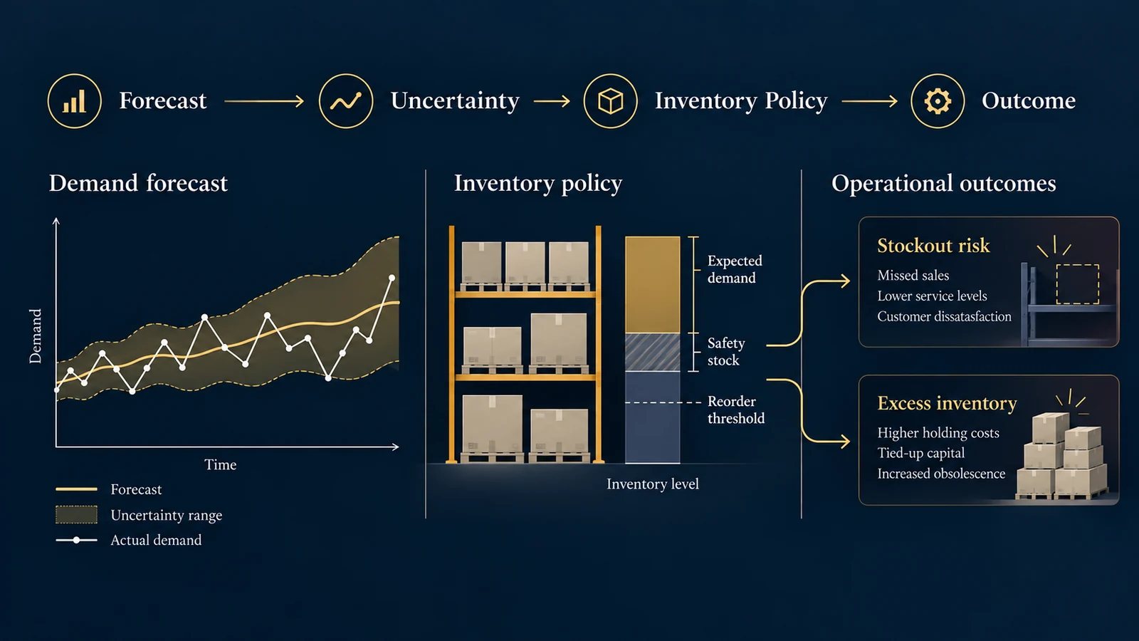
A retailer invests in a new demand forecasting system. The model performs well during testing, with relatively low average forecasting error. Management expects fewer stockouts, lower inventory costs, and better purchasing decisions.
Three months later, however, the company still experiences product shortages. Some items run out unexpectedly; others remain in storage longer than anticipated.
The forecasting model may be performing as designed. So why are the inventory outcomes disappointing?
Because predicting demand and deciding how much inventory to hold are two different analytical problems.
A demand forecast estimates future demand. An inventory policy determines what the organization should do given that forecast, the uncertainty surrounding it, replenishment constraints, and the consequences of being wrong.
A forecast can be statistically accurate without producing an economically effective inventory decision. Understanding that gap is the starting point for better inventory analytics.
Forecast Accuracy Is Not the Same as Inventory Performance
Demand forecasting models are commonly evaluated using statistical error measures such as Mean Absolute Error (MAE), Root Mean Squared Error (RMSE), Mean Absolute Percentage Error (MAPE), and Mean Absolute Scaled Error (MASE). They describe different aspects of forecast performance. For example, MAE measures the average absolute difference between predicted and observed demand, while RMSE gives greater weight to larger errors.
MAPE expresses errors relative to actual values, but is undefined when actual demand is zero and unstable when actual demand is close to zero. Forecasting: Principles and Practice discusses these metric properties and the importance of evaluating genuine forecast performance.
None of these measures directly tells a business when to reorder, how much safety stock to maintain, how frequently shortages may occur, how much working capital inventory requires, or whether the inventory policy is economically appropriate.
Those are decision questions. Forecasting provides inputs; inventory optimization determines actions.
The Missing Variable: Forecast Uncertainty
Suppose a company forecasts demand of 100 units tomorrow. What does that prediction mean?
It might describe a product whose demand is usually between 95 and 105 units. Or it might describe a product whose demand frequently fluctuates between 50 and 150 units. Both products can have the same point forecast, but their inventory requirements may be very different.
A point forecast provides a central estimate. A forecast distribution describes uncertainty around that estimate. This is why probabilistic forecasting can be more useful than point forecasting for operational decisions.
For example, a forecasting system might estimate expected demand of 100 units and a plausible range of 70–130 units. That range is illustrative; it is not a calibrated prediction interval unless a probability level and valid forecasting method are specified. Hyndman and Athanasopoulos explain how distributional forecasts and prediction intervals represent uncertainty across possible future values in Forecasting: Principles and Practice, Section 5.5.
The relevant question becomes: How much demand should we prepare for, given the cost of shortages and the cost of excess inventory? That question leads directly to safety stock and replenishment decisions.
What Is Safety Stock?
Safety stock is inventory held to protect against uncertainty. Uncertainty can arise from demand fluctuations, supplier delays, production variability, transportation disruptions, forecasting errors, and other operational factors. Safety stock is not necessarily evidence of inefficient inventory management; it can be a deliberate response to uncertainty.
However, excessive safety stock ties up capital and increases storage, financing, and obsolescence costs. Insufficient safety stock increases exposure to stockouts. The objective is not to maximize or minimize safety stock independently, but to choose a policy appropriate for service requirements, operating constraints, and economics. MIT's logistics course and IBM's overview both discuss safety stock as part of a broader inventory and replenishment problem (MIT OpenCourseWare: Logistics Systems, Lecture 11; IBM: What Is Safety Stock?).
A Worked Example: Calculating a Reorder Point
Consider a hypothetical retailer selling one product. Assume average daily demand is 100 units, the standard deviation of daily demand is 20 units, supplier replenishment lead time is seven days, and the target cycle service level is 95%.
For this example, assume daily demand is independent across days, demand follows a stable distribution, the daily demand standard deviation remains constant, lead time is fixed at seven days, demand during lead time is approximately normally distributed, inventory is reviewed continuously, replenishment is reliable, and the standard continuous-review reorder-point assumptions apply. These assumptions simplify the mathematics; they should not be presumed to hold in a real business.
Step 1: Calculate expected demand during lead time
The business expects to sell 100 units per day, and the supplier requires seven days to replenish inventory:
If demand were perfectly predictable, 700 units would cover the expected replenishment period. But demand is uncertain.
Step 2: Calculate lead-time demand variability
Under the independent, identically distributed daily-demand assumptions:
This calculation depends on independence. If demand errors are positively correlated across days, uncertainty may accumulate more rapidly. Seasonal demand, trends, and promotions may require a different model.
Step 3: Select a cycle service target
Suppose management chooses a 95% cycle service target. Under the normal approximation, the corresponding one-sided standard normal quantile is approximately z = 1.645.
A 95% cycle service target represents a modeled 95% probability of avoiding a stockout during a replenishment cycle under the specified inventory-policy assumptions. It does not mean that 95% of all customer demand units will necessarily be fulfilled; that latter concept relates to fill rate, a different measure.
Step 4: Calculate safety stock
For whole-unit inventory, the company rounds the resulting reorder threshold upward.
Step 5: Calculate the reorder point
Under this illustrative continuous-review policy, the business places a replenishment order when its inventory position reaches or falls below the reorder threshold. Inventory position is generally defined as:
This is not the same as checking only the units physically on warehouse shelves. Outstanding purchase orders and unfulfilled customer orders matter. The reorder point determines when to order; it does not by itself determine the order quantity.
How the Service Target Changes Inventory Requirements
The service target affects the amount of safety stock. Using the same hypothetical product—expected lead-time demand 700 units and lead-time demand standard deviation 52.92 units—compare three cycle service targets:
| Cycle Service Target | Approx. Z-Value | Safety Stock, Rounded Up | Reorder Point |
|---|---|---|---|
| 90% | 1.282 | 68 units | 768 units |
| 95% | 1.645 | 88 units | 788 units |
| 99% | 2.326 | 124 units | 824 units |
All values are illustrative model calculations. Increasing the target from 90% to 95% raises the reorder point by 20 units; moving from 95% to 99% adds another 36 units. Higher service targets generally require more inventory under this model, but the business must decide whether additional protection is worth the carrying cost. That is an economic decision, not simply a forecasting decision.
What Does Additional Safety Stock Cost?
Suppose annual inventory holding cost is $30 per unit. This is the estimated annual cost of carrying one additional unit, not the product's selling price. Moving from the 95% to the 99% cycle service target increases safety stock by:
The approximate additional annual holding cost is:
For one product, that may be manageable. Across 1,000 comparable products, the same increase would imply:
in additional annual holding cost, assuming the incremental average inventory and holding-cost parameters apply similarly to each product. This excludes potential benefits from fewer shortages as well as other operational effects such as ordering costs, supplier constraints, or obsolescence. It illustrates why service-level decisions should be connected to inventory economics rather than automatically setting the highest possible target for every item.
Cycle Service Level Is Not the Same as Fill Rate
Inventory discussions often use “service level” without defining it. Two common measures are:
- Cycle service level: the probability of avoiding a stockout during a replenishment cycle under the inventory model.
- Fill rate: the proportion of demand units fulfilled directly from available inventory, using the organization's defined measurement.
Consider a product that stocks out during one replenishment cycle. If only one unit is unavailable, the effect on unit fill rate may be small. If hundreds of units are unavailable, the effect may be substantial. Both situations can count as stockout cycles. Therefore, the same cycle service level can correspond to different fill rates.
Management should explicitly choose the measure that represents its operational objective. The distinction is important when comparing policies or reporting performance across departments.
Why Lead Time Matters as Much as Forecast Accuracy
Return to the example. Daily demand and its standard deviation remain 100 and 20 units, and the cycle service target remains 95%. But suppose supplier lead time increases from seven days to fourteen days.
The required reorder threshold has increased substantially even though the forecasting model did not change. The difference comes from the replenishment process. Improving supplier reliability, reducing lead times, and improving forecasts can be complementary strategies; forecasting is not the only way to improve inventory performance.
What If Supplier Lead Time Is Uncertain?
The preceding calculations assumed fixed lead time. Real suppliers may deliver earlier or later than expected. Under a simplified model where daily demands are independent and identically distributed, lead time is independent of demand, and the required moments exist:
Here, DLT is demand accumulated during lead time, L is lead time, μD is average daily demand, and σD is the standard deviation of daily demand. The approximation illustrates why supplier reliability can affect inventory requirements.
It should not be used blindly. Lead-time demand may be affected by seasonal patterns, supplier disruptions, correlated demand, promotions, holidays, or dependencies between demand and replenishment delays. Historical lead-time demand distributions or simulation may be more suitable in complex settings. MIT's inventory teaching material provides further context on lead-time demand variability and the square-root relationship under simplifying assumptions (MIT, Inventory Basics).
Two Forecasts Can Have the Same MAE but Different Inventory Implications
Consider four hypothetical periods. Actual demand is 90, 110, 90, and 110 units. Two models produce these predictions:
| Period | Actual Demand | Model A | Model B |
|---|---|---|---|
| 1 | 90 | 100 | 80 |
| 2 | 110 | 100 | 100 |
| 3 | 90 | 100 | 80 |
| 4 | 110 | 100 | 100 |
For Model A, forecast errors defined as actual minus predicted are −10, +10, −10, and +10. Its MAE is 10 units and its mean signed error is 0. For Model B, errors are +10 in all four periods. Its MAE is also 10 units, but its mean signed error is +10 units.
Model B consistently underforecasts in this small example. If inventory decisions use these forecasts without accounting for the bias, the shortage exposure may differ. The example does not prove Model A always produces a better policy: outcomes also depend on uncertainty estimates, replenishment rules, order quantities, and costs. It shows that a single accuracy statistic can conceal operationally relevant differences.
Forecast Bias Deserves Its Own Metric
Forecast bias describes systematic overprediction or underprediction. Using the convention:
Positive mean error indicates underforecasting; negative mean error indicates overforecasting. A useful reporting system can track MAE, RMSE, mean signed error, forecast error by product, by season, and by forecast horizon.
A model can have low average absolute error while consistently missing demand in one direction. That matters when the consequences of underforecasting and overforecasting are asymmetric. Underforecasting may create lost sales, delayed fulfillment, customer dissatisfaction, and emergency replenishment costs. Overforecasting may create excess inventory, storage costs, working-capital requirements, markdowns, and obsolescence. Their relative importance varies by product and business.
The Forecast Horizon Must Match the Decision
A business may report, “Our one-day-ahead forecasting model is highly accurate.” But its suppliers require fourteen days to deliver inventory. The operational decision depends on demand during replenishment, not merely tomorrow's demand.
A model evaluated only on one-day-ahead predictions may not provide sufficient evidence about fourteen-day cumulative demand. The evaluation horizon should reflect replenishment frequency, supplier lead time, planning horizon, and the timing of inventory decisions. For periodic-review policies, the protection period can include both the review interval and replenishment lead time.
Evaluate Forecasts Using Historical Decision Points
A forecasting model should be tested using information that would actually have been available when each historical decision was made. Rolling-origin backtesting is one way to do this:
- Use data available through January to forecast February.
- Compare the forecast with observed February demand.
- Move the forecasting origin forward.
- Use data available through February to forecast March.
- Repeat across historical periods.
The evaluation should not allow future information to leak into earlier predictions. Hyndman and Athanasopoulos' discussion of time-series cross-validation explains rolling-origin evaluation and how forecast horizon affects assessment.
For inventory decisions, evaluation can go further. At each historical origin, generate the demand forecast, estimate uncertainty, calculate the reorder threshold, apply or simulate the policy, and evaluate resulting costs and service outcomes. This is more decision-relevant than comparing forecasting error alone.
A Critical Data Problem: Sales Are Not Always Demand
Suppose a store sells 100 units of a product and then runs out. Its transaction system records 100 units sold. But was actual customer demand 100, 120, or 200? Sales data alone cannot determine how many customers wanted the product after it became unavailable. This is known as censored demand.
If a company trains a demand model directly on sales without accounting for stockouts, the model may learn artificially low demand during periods when products were unavailable. It may forecast low demand, stock fewer units, sell out, record low sales, and then forecast low demand again.
Breaking this cycle requires more than selecting a sophisticated algorithm. Useful information may include inventory availability, stockout timestamps, backorders, abandoned orders, lost-sales estimates, substitute purchases, and other demand signals. These signals require careful interpretation; not every abandoned purchase represents demand that would have converted. The goal is to distinguish observed sales from underlying customer demand as credibly as possible.
Reliable transaction, availability, and product records matter here. See this related guide to data quality checks in analytics pipelines.
When Should Businesses Use Probabilistic Forecasting?
Point forecasts are useful when the primary objective is to estimate a central expected outcome. Probabilistic forecasts become especially valuable when decisions depend on uncertainty, including inventory replenishment, staffing, capacity planning, transportation, cash-flow planning, and risk management.
Instead of producing only expected demand of 100 units, a probabilistic model can estimate a distribution of possible demand and quantiles such as the 10th, 50th, or 90th percentile. Those quantities can support decisions with different risk tolerances.
Prediction intervals and quantiles must be evaluated for calibration. A nominal 90% interval should contain approximately 90% of future observations over a sufficiently representative evaluation sample if it is well calibrated; coverage should be checked rather than assumed. The distribution must also match the decision horizon. A well-calibrated one-day demand interval is not automatically a well-calibrated fourteen-day cumulative-demand interval.
Should Every Business Use Machine Learning?
Not necessarily. A sophisticated forecasting model can help when demand patterns depend on many interacting variables such as price changes, promotions, holidays, weather, product characteristics, geography, and complex seasonality. But more complex models also require reliable data, appropriate validation, monitoring, maintenance, and operational integration.
A simple seasonal method may outperform a poorly implemented machine-learning model. The right question is not “Can we build a more advanced forecast?” but “Will an improved forecast produce a sufficiently valuable improvement in the decisions we make?” That requires evaluating the complete decision system, including turning predictive analytics into decisions.
A Better Inventory Analytics Scorecard
An effective inventory dashboard connects forecasting performance with operational outcomes:
| Dimension | Example Metrics | Management Question |
|---|---|---|
| Forecast Accuracy | MAE, RMSE, MASE | How closely do predictions match demand? |
| Forecast Bias | Mean signed error | Are we systematically over- or underforecasting? |
| Uncertainty | Interval coverage, lead-time demand distribution | Are uncertainty estimates calibrated? |
| Inventory Policy | Reorder points, safety stock, order quantities | Are replenishment rules appropriate? |
| Service | Cycle service level, fill rate, backorders | Are customers receiving products when needed? |
| Financial Impact | Holding costs, shortage costs, markdowns | Is the policy economically effective? |
| Supply Reliability | Actual lead time, lead-time variability | Are suppliers meeting operational expectations? |
These metrics answer different questions and should not be collapsed into one forecasting accuracy score. A company may improve MAE while inventory holding costs increase. Another may accept slightly larger errors while achieving better service and lower total costs through a more appropriate policy. The complete operational result matters.
A Practical Implementation Framework
1. Define the inventory decision
Determine what management needs to decide: when to place an order, how much to order, what service target is appropriate, which products require more safety stock, or which suppliers create the greatest replenishment uncertainty. The decision determines the necessary data and analytical methods.
2. Establish reliable demand data
Combine relevant information from sales, inventory, purchasing, supplier, product-catalog, and promotional systems. Investigate missing transactions, duplicate records, product identifier inconsistencies, stockout periods, returns, and changes in product availability. Data-quality problems can undermine sophisticated forecasting methods.
3. Forecast at the correct granularity
Determine whether the relevant level is product, store, warehouse, region, or category. Forecasting total company demand may be insufficient when inventory must be allocated to individual locations, while overly granular forecasts can become noisy. The appropriate level depends on the replenishment decision and available data.
4. Quantify uncertainty
Evaluate more than point-forecast accuracy. Estimate bias, forecast-error variability, interval coverage, lead-time demand uncertainty, and supplier lead-time variability; validate the estimates using historical data.
5. Evaluate alternative inventory policies
Compare reorder points, service targets, order quantities, replenishment frequencies, and supplier strategies. For complex systems, simulation can incorporate uncertain demand, supplier delays, multiple products, warehouse constraints, and alternative rules. It estimates how policies perform under explicitly modeled assumptions; it does not guarantee future outcomes. The appropriate modeling approach depends on the decision, and scenario analysis and Monte Carlo simulation can help frame different types of uncertainty.
6. Monitor business outcomes
After implementation, track stockouts, achieved service levels, holding costs, replenishment performance, and other operational outcomes. Compare results with original assumptions and update models and policies when evidence indicates demand patterns, supplier performance, or business requirements have changed.
Correlation, Attribution, and Causality
Suppose a business introduces a new forecasting system. Six months later, forecast MAE is lower, stockouts have declined, and inventory holding costs have decreased. Those changes are encouraging, but do not by themselves establish that the forecasting system caused every improvement.
Supplier reliability, staffing, product mix, replenishment frequency, purchasing policies, or customer demand may also have changed. Observed results describe what happened. A causal evaluation asks what would have happened without the new system.
Depending on feasibility, stronger designs may include randomized rollouts across comparable products or locations, controlled pilots, difference-in-differences, or interrupted time-series analysis with appropriate assumptions. Even when causal identification is not possible, transparent observational reporting is useful. The key is not to present association as proof of causation.
What Should Management Actually Optimize?
A company should not optimize forecasting accuracy in isolation. A more useful objective is often to minimize the expected total cost of inventory decisions while meeting appropriate service and operational constraints.
Relevant costs may include holding, ordering, transportation, shortages, lost sales, emergency replenishment, and obsolescence. Some costs are difficult to estimate; customer dissatisfaction and long-term reputation effects may be especially uncertain. The objective function should therefore be documented clearly.
Service targets should reflect product importance. A low-margin, easily substitutable product may justify a different policy from a critical product with severe shortage consequences. There is no universally optimal safety-stock percentage or reorder point. The correct policy depends on demand uncertainty, replenishment behavior, service requirements, and business economics.
The Real Value of Forecasting Is Better Decisions
An accurate forecast is valuable, but it is not the final outcome. A forecasting system becomes operationally useful when its estimates are connected to uncertainty, replenishment constraints, service targets, inventory economics, and clearly defined decisions.
This sequence moves forecasting beyond statistical performance. It helps organizations understand not only what demand may look like, but also how they should prepare for it.
A business does not ultimately benefit from a forecasting model because its error statistic is impressive. It benefits when the model contributes to better inventory availability, more efficient resource allocation, and more defensible operational decisions. Explore UAD's predictive analytics and modeling services for support connecting analytical results to operational choices.
References
- Hyndman, Rob J., and George Athanasopoulos. Forecasting: Principles and Practice, 3rd ed., Section 5.5, “Distributional Forecasts and Prediction Intervals.” otexts.com/fpp3/prediction-intervals.html.
- Hyndman, Rob J., and George Athanasopoulos. Forecasting: Principles and Practice, 3rd ed., Section 5.8, “Evaluating Point Forecast Accuracy.” otexts.com/fpp3/accuracy.html.
- Hyndman, Rob J., and George Athanasopoulos. Forecasting: Principles and Practice, 3rd ed., Section 5.10, “Time Series Cross-Validation.” otexts.com/fpp3/tscv.html.
- MIT OpenCourseWare. Logistics Systems, Lecture 11, “Inventory Management, Probabilistic Demand, and Safety Stock.” MIT OpenCourseWare.
- IBM. “What Is Safety Stock?” IBM Think.
- MIT. “Inventory Basics.” Course lecture material (PDF).
Turn Better Forecasts Into Better Business Decisions
UAD Consulting helps organizations connect predictive analytics, data modeling, and decision analysis to practical business questions. From demand forecasting to scenario evaluation, the goal is to translate analytical results into more informed operational decisions.
Explore ServicesGet in Touch