A financial model says a project will generate a $1.2 million return.
That number may be mathematically correct.
It can still be a poor description of the decision.
The result depends on assumptions: demand, price, cost, adoption, conversion, project duration, inflation, retention, or other uncertain inputs.
Change those assumptions and the answer changes.
The practical question is therefore not only:
“What is the expected result?”
It is also:
“How uncertain is that result, and could the uncertainty change the decision?”
Two common ways to answer that question are scenario analysis and Monte Carlo simulation.
They are related, but they solve different analytical problems.
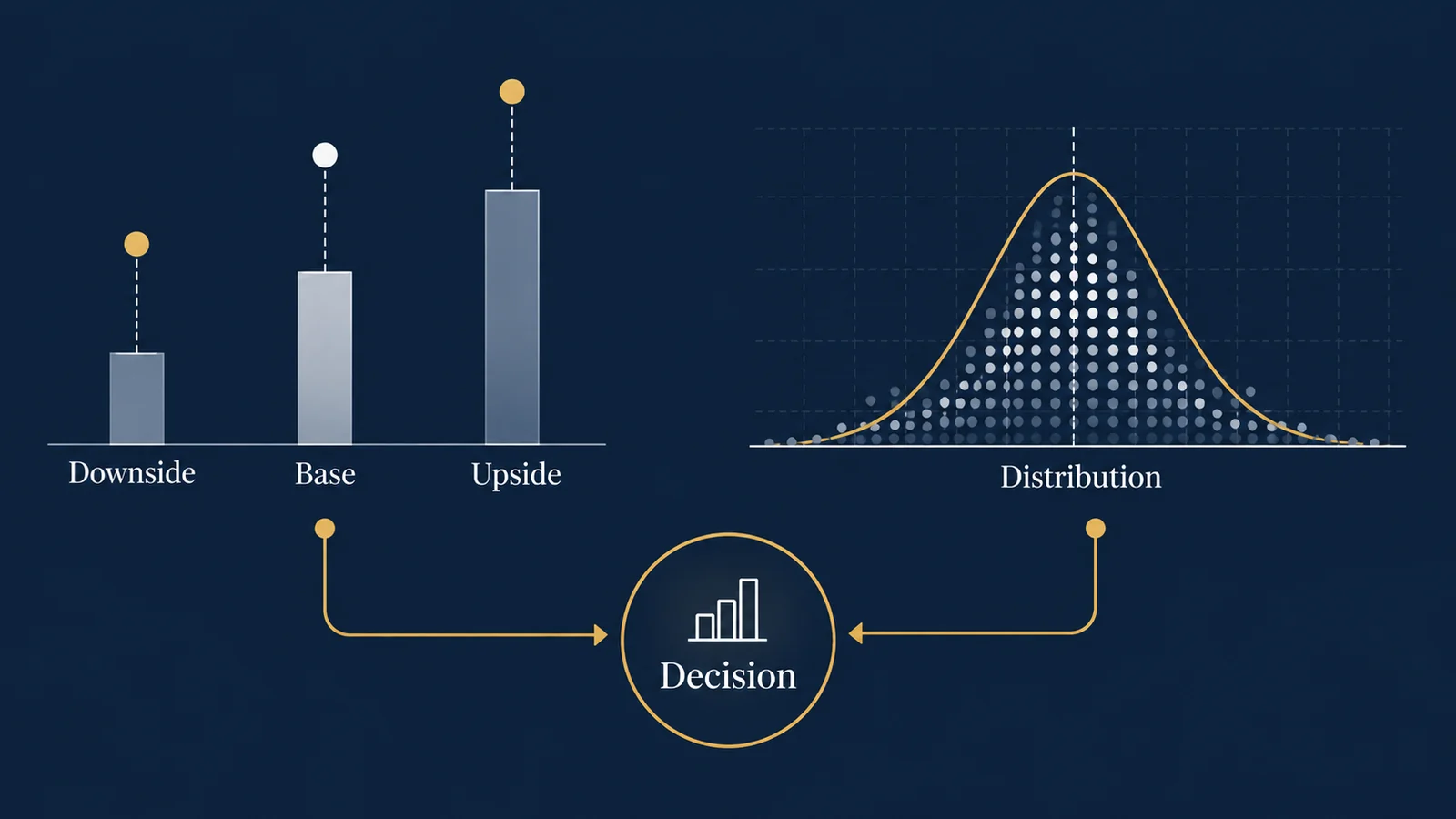
Scenario analysis evaluates a small number of deliberately chosen combinations of assumptions. Monte Carlo simulation repeatedly samples uncertain inputs from specified probability distributions and produces a distribution of possible model outcomes.
Neither method is automatically better. The right method depends on the decision, the uncertainty, the available evidence, and how much analytical complexity is justified.
- Selected futures
- Uncertain inputs
- Model outcomes
- Decision thresholds
What Is Scenario Analysis?
Scenario analysis asks:
What happens if a particular set of assumptions occurs?
A business might construct three cases:
- downside,
- base case,
- upside.
Suppose a company is evaluating a new service. The model depends on annual customers, revenue per customer, variable cost per customer, and annual fixed cost.
The basic contribution model is:
Annual Profit = Customers × (Revenue per Customer − Variable Cost per Customer) − Fixed Cost
| Assumption | Downside | Base Case | Upside |
|---|---|---|---|
| Customers | 6,000 | 8,000 | 10,000 |
| Revenue/customer | $190 | $200 | $210 |
| Variable cost/customer | $130 | $125 | $120 |
| Fixed cost | $500,000 | $500,000 | $500,000 |
Now calculate each outcome.
Downside:
6,000 × ($190 − $130) − $500,000 = -$140,000
Base case:
8,000 × ($200 − $125) − $500,000 = $100,000
Upside:
10,000 × ($210 − $120) − $500,000 = $400,000
The analysis now tells management something the single $100,000 base-case estimate did not. Under the selected assumptions, outcomes range from a $140,000 loss to a $400,000 profit.
That is useful. But it still leaves several questions unanswered. How likely is each scenario? What happens between them? Could outcomes outside those three cases occur? And what if some uncertain variables move independently rather than all improving or deteriorating together?
What Scenario Analysis Does Well
Scenario analysis is especially useful when the decision maker wants to understand a small number of interpretable futures.
It works well for questions such as:
- What if adoption is 20% below plan?
- What if costs increase while demand stays flat?
- What if a competitor enters the market?
- What if reimbursement changes?
- What if a marketing budget is cut?
- What if implementation is delayed six months?
The method is transparent. A manager can inspect the assumptions and understand exactly why the result changed. That makes scenario analysis useful for communication and decision workshops.
It is also relatively easy to implement in spreadsheets, SQL-driven models, BI tools, or financial planning systems. Microsoft Power BI supports numeric parameters that can be incorporated into measures and controlled interactively through report slicers, allowing report users to change assumptions and observe how outputs respond.
But interactive parameters are still not the same thing as probabilistic simulation. A user moving a slider is choosing assumptions. A Monte Carlo model samples assumptions according to specified probability distributions.
What Is Monte Carlo Simulation?
Monte Carlo simulation asks a different question:
What range of outcomes could the model produce when uncertain inputs vary according to specified probability distributions?
Instead of assigning demand one downside value, one base value, and one upside value, an analyst specifies a distribution.
Revenue per customer: Normal distribution; mean = $200; standard deviation = $8
Variable cost per customer: Triangular distribution; minimum = $115; most likely = $125; maximum = $140
The model then repeatedly samples values from these distributions.
One simulated iteration might produce customers = 7,420, revenue/customer = $203, and variable cost/customer = $128.
7,420 × ($203 − $128) − $500,000 = $56,500
Another iteration might produce customers = 6,350, revenue/customer = $192, and variable cost/customer = $134.
6,350 × ($192 − $134) − $500,000 = -$131,700
Repeat this process thousands of times and the output is no longer one forecast. It is a distribution of forecasts.
NIST describes Monte Carlo analysis as a probabilistic sensitivity analysis in which uncertain inputs are assigned probability distributions and repeatedly sampled to propagate uncertainty through a model.
The Difference in One Table
| Question | Scenario Analysis | Monte Carlo Simulation |
|---|---|---|
| How many futures are evaluated? | Usually a small selected set | Hundreds or thousands of simulated outcomes |
| Inputs | Fixed values for each scenario | Probability distributions |
| Output | Discrete outcomes | Distribution of outcomes |
| Easy to explain? | Very | Moderate |
| Captures intermediate combinations? | Limited | Yes |
| Estimates probability of loss? | Not inherently | Yes, conditional on model assumptions |
| Requires probability assumptions? | No | Yes |
| Useful for risk quantification? | Limited | Stronger |
Three scenarios do not become a probability model merely because they are labeled downside, base, and upside.
A Three-Scenario Model Can Hide Risk
Return to the service example. The three scenarios produced downside -$140,000, base $100,000, and upside $400,000.
A manager might look at these values and conclude that the project is attractive because two of the three scenarios are profitable. That conclusion would be invalid.
The three scenarios do not necessarily have equal probability. Counting profitable scenarios is not the same as estimating the probability of profit. If the downside assumptions are much more likely than the upside assumptions, the decision could look very different.
What a Monte Carlo Result Can Tell You
Suppose an analyst runs 50,000 simulated iterations of a properly specified model.
| Metric | Simulated Result |
|---|---|
| Mean annual profit | $112,000 |
| Median annual profit | $97,000 |
| 10th percentile | -$105,000 |
| 90th percentile | $355,000 |
| Probability of loss | 27% |
| Probability profit exceeds $250,000 | 19% |
These are illustrative results, not empirical estimates for a real company. But notice how the decision conversation changes. Instead of saying “The project should make approximately $100,000,” management can discuss: “The model's central outcome is around $100,000, but under our stated uncertainty assumptions approximately 27% of simulated outcomes produce a loss.”
Expected Value Is Not the Whole Decision
Suppose two projects have the same expected profit: Project A and Project B both equal $150,000. But Project A has a 5% probability of loss while Project B has a 35% probability of loss.
A risk-neutral decision maker focused purely on expected value might treat them similarly. A cash-constrained business might not. The organization may care about probability of loss, probability of exceeding a minimum return, downside percentile, cash required before break-even, probability of exceeding capacity, or another decision-specific threshold.
Decision analytics should not automatically reduce uncertainty to a single average. The relevant output depends on what would actually change the decision.
Probability of Loss Is Often More Actionable Than a Range
A traditional model might report expected profit of $120,000 and a range of -$200,000 to $500,000. The range is informative but incomplete.
A Monte Carlo model can estimate P(Profit < 0) by dividing the number of simulations with negative profit by total simulations. If 6,750 of 25,000 outcomes are negative, the probability of loss under the model assumptions is 27%.
The phrase “under the model assumptions” matters. Monte Carlo simulation does not discover the true probability of loss automatically. It calculates outcomes implied by the probability distributions, dependencies, formulas, and assumptions supplied to the model.
Monte Carlo Simulation Does Not Remove Assumptions
A simulation does not replace subjective assumptions with objective probability. Suppose demand is modeled as a normal distribution with mean 8,000 and standard deviation 1,000. Those values may come from historical data, experiments, market research, expert judgment, forecasting models, or a combination.
The quality of the simulation depends on the quality and appropriateness of those inputs. Simulation makes uncertainty explicit; it does not make uncertainty disappear.
Choosing the Distribution Matters
Triangular Distribution
Useful when the analyst can reasonably specify minimum, most likely, and maximum values. It is practical when data is limited but domain knowledge can define plausible bounds.
Normal Distribution
Useful for some approximately symmetric uncertain quantities. But it extends theoretically without bounds, so it can be inappropriate for variables that cannot be negative or have hard limits.
Uniform Distribution
Assigns equal density across a specified range. It can be useful when bounds are known but there is insufficient basis for identifying more likely values within the range.
NIST identifies triangular, normal, and uniform distributions among common choices and emphasizes defining the variables, distributions, and number of simulation iterations. The correct distribution should reflect evidence and the structure of the problem rather than whichever is easiest to implement.
Correlation Between Inputs Can Change the Risk
Suppose price and demand are uncertain. If higher prices tend to reduce demand, treating them as independent can generate unrealistic combinations such as very high price plus very high demand too frequently. Material costs and transportation costs might also increase together.
Ignoring dependency can distort the output distribution. A mature simulation asks whether uncertain inputs are independent and what correlation or dependency structure is defensible. NIST's Uncertainty Machine supports correlated inputs when propagating uncertainty through models.
This illustrates an important principle: the marginal distribution of each input is not the entire uncertainty model.
Sensitivity Analysis and Monte Carlo Simulation Are Not the Same Thing
Sensitivity analysis asks: Which assumptions have the greatest influence on the result? Monte Carlo simulation asks: What distribution of outcomes results from uncertain inputs?
They are complementary. After running a simulation, an analyst may discover that profit uncertainty is primarily associated with customer adoption, variable cost, price, and implementation delay. If adoption uncertainty dominates, additional market research might be more valuable than refining a minor cost assumption.
NIST decision-support guidance has used a progression from baseline analysis to sensitivity analysis and then Monte Carlo simulation to evaluate uncertainty and financial risk.
When Scenario Analysis Is Enough
Monte Carlo simulation is not necessary for every decision. Scenario analysis may be sufficient when the decision has only a few important uncertainties, management wants specific strategic states, probability distributions would be mostly arbitrary, the model is primarily for communication, the decision is easily reversible, or the cost of a wrong decision is relatively small.
For example, a manager deciding whether to add one analyst next quarter may get enough value from a base case, a high-demand case with 20% more projects, and a low-demand case with 20% fewer projects. Building a 100,000-iteration simulation would not automatically make the staffing decision better.
When Monte Carlo Simulation Adds Value
Simulation becomes more useful when several uncertain variables interact, downside risk matters, thresholds matter, the decision is expensive or difficult to reverse, management needs probability-based risk measures, uncertainty compounds over time, or deterministic scenarios hide too many possible combinations.
Examples can include capital investment, inventory planning, capacity planning, project cost risk, demand planning, financial forecasting, health economic modeling, budget impact analysis, and operational risk analysis. The common feature is not the industry; it is that uncertainty can materially alter the preferred decision.
A Decision Rule Is Better Than “Run the Model”
A simulation is most useful when it connects to an explicit decision. Suppose management will launch only if probability of loss is below 20% and probability of earning at least $200,000 is above 40%.
If the output is P(Loss) = 27% and P(Profit ≥ $200,000) = 31%, the project would not qualify under the stated rule. Management could reduce fixed cost, increase price, pilot the service, improve demand evidence, renegotiate variable costs, or change the risk threshold.
The model has moved from forecasting to decision support.
Expected Value Can Also Support Choices Between Alternatives
Suppose Strategy A has a 60% chance of $300,000 profit and a 40% chance of a $50,000 loss.
0.60 × $300,000 + 0.40 × -$50,000 = $160,000
Strategy B has a 90% chance of $160,000 profit and a 10% chance of a $20,000 loss.
0.90 × $160,000 + 0.10 × -$20,000 = $142,000
Strategy A has the higher expected value. That does not automatically make it correct. The organization may value Strategy B's lower downside risk. Decision analysis separates what the model predicts from what the decision maker values.
Simulation Does Not Establish Causality
This distinction matters when uncertain inputs come from observational data. If historical analysis shows that customers receiving an intervention have higher retention, that association can be incorporated into a scenario model. But simulation does not transform association into a causal effect.
If the underlying estimate is confounded, repeatedly sampling it does not remove the confounding. Monte Carlo simulation propagates uncertainty through a model; it does not establish that changing an input will causally produce the modeled outcome.
Causal claims require an appropriate research design, experiment, quasi-experimental method, or defensible causal model. This is the broader analytical principle behind correlation and causation in business decisions.
Scenario Analysis Can Be the First Layer of a Simulation Model
The two approaches should not always be treated as competitors. A useful progression is:
- Point Estimate
- Scenario Analysis
- Sensitivity Analysis
- Probabilistic Simulation
- Decision Rule
A team might first create three scenarios to understand the structure of the problem, then perform sensitivity analysis to identify important assumptions, and only then assign probability distributions to the important uncertain inputs. This prevents unnecessary complexity and helps stakeholders understand the model before probabilistic results are introduced.
A Practical Framework for Choosing the Method
Use five questions.
1. How many uncertainties materially affect the decision?
One or two: scenario analysis may be sufficient. Several interacting uncertainties: simulation becomes more attractive.
2. Do probabilities matter?
If management only needs several strategic cases, scenarios may work. If management asks “What is the probability we lose money?” a probabilistic model is required to answer quantitatively.
3. Can the uncertainty distributions be defended?
A simulation with arbitrary distributions can create false precision. If evidence is weak, transparent scenarios may be more honest.
4. How costly is the decision?
More consequential and irreversible decisions can justify greater analytical effort.
5. What action will change because of the result?
If no plausible model output would change the decision, more simulation may have little practical value. The purpose is not to build the most sophisticated model. It is to improve the decision.
What Should a Decision Dashboard Show?
A decision dashboard should not bury uncertainty behind a single KPI. For a simulation-based decision, useful outputs can include expected outcome, median outcome, downside percentile, upside percentile, probability of loss, probability of meeting the target, key sensitivity drivers, and comparison across decision alternatives.
A useful visual layout might contain decision assumptions, a distribution of simulated outcomes, and decision thresholds with the probability of meeting them. This is different from a conventional performance dashboard: the purpose is to support a decision about what to do next. See which KPIs belong on a dashboard for a decision-first dashboard perspective.
A Model Should Expose Its Assumptions
A decision model should make visible its objective, alternatives, uncertain inputs, source of each assumption, probability distributions, correlations, formulas, simulation count, decision thresholds, and limitations.
This matters because simulation outputs can appear authoritative. A histogram containing 50,000 iterations is still conditional on the assumptions that generated those iterations. More iterations reduce simulation noise; they do not repair a poorly specified model.
From Forecasting to Decision Analytics
Forecasting asks: What might happen?
Decision analytics goes further: What should we do given what might happen, our objectives, and our constraints?
Scenario analysis and Monte Carlo simulation are tools in that process. Scenario analysis provides interpretable alternative futures. Monte Carlo simulation provides a probabilistic representation of uncertainty when assumptions can be reasonably specified. Sensitivity analysis identifies which assumptions matter most. Decision rules connect the model to action.
- Define Decision
- Identify Uncertainty
- Build Baseline
- Test Scenarios
- Analyze Sensitivity
- Simulate When Justified
- Apply Decision Rule
- Act
The goal is not to eliminate uncertainty. No model can do that. The goal is to make uncertainty visible enough that the organization can make a better decision.
References / Further Reading
- NIST — Monte Carlo Tool
- NIST — Incorporating Attribute Value Uncertainty into Decision Analysis
- NIST — Users Manual for Version 4.0 of the Cost-Effectiveness Tool for Capital Asset Protection
- Microsoft Learn — Create and use parameters to visualize variables in Power BI Desktop
- NIST — Uncertainty Machine
Turn Uncertainty Into a Better Decision
UAD Consulting helps businesses structure decision models, evaluate uncertainty, and translate analytical results into practical choices.