A healthcare organization is evaluating a new treatment. Clinical evidence suggests the treatment may reduce complications, but it costs more than the existing alternative. Management wants to know whether the additional health benefit justifies the additional expenditure.
The analytics team proposes a cost-effectiveness model. One analyst recommends a decision tree. Another recommends a Markov model. Which approach is appropriate?
The answer depends less on the sophistication of the software and more on the clinical process being represented. A decision tree is often suitable for relatively short, well-defined sequences of events. A Markov model is generally more useful when patients can move repeatedly between health states over time.
Neither method is automatically superior. The correct model is the simplest structure capable of representing the important differences between the interventions being compared. That principle is consistent with ISPOR-SMDM good research practices guidance on model conceptualization and state-transition modeling [1, 2].
What Is a Decision Tree in Health Economics?
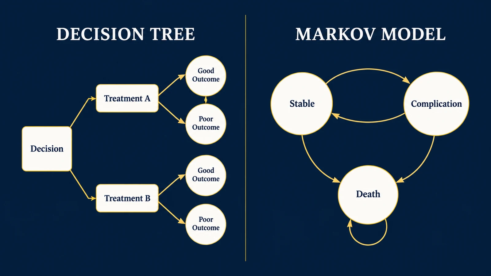
A decision tree represents a sequence of decisions, events, and possible outcomes. The structure begins with a decision. Each alternative leads to branches representing possible consequences. Probabilities describe how patients move through the branches. Costs and health outcomes are assigned to the resulting pathways.
Consider a hypothetical diagnostic strategy. A healthcare organization must choose between standard diagnostic testing and a new diagnostic test. Each strategy can produce a positive or negative result. Depending on the patient's true condition, those results may be correct or incorrect. The model can calculate expected costs and consequences across the pathways.
The same principle can be used for expected health outcomes. Decision trees are particularly useful when the decision has a limited number of clinically meaningful branches and consequences can be represented within a manageable time horizon.
Examples include short-term diagnostic pathways, immediate procedural complications, one-time screening decisions, acute treatment decisions, and short-term adverse-event comparisons.
However, decision trees become increasingly cumbersome when the same events can occur repeatedly. A chronic disease model may require patients to experience complications, recover, relapse, and experience additional complications over many years. Representing every possible sequence as a separate branch can become impractical. This is where state-transition modeling is useful.
What Is a Markov Model?
A Markov model represents a system using a defined set of states and the probabilities of moving between those states over time. In health economics, the states often represent clinically meaningful health conditions.
For example, a model might include Stable health, Complication, and Death. Patients begin in one state. During each model cycle, they may remain in their current state or transition to another. A cycle might represent one month, three months, six months, or one year. The appropriate cycle length depends on the clinical process and timing of important events.
A cohort Markov model follows the expected distribution of a population across states. An individual-level state-transition model follows simulated patients. Both belong to the broader family of state-transition models described in ISPOR-SMDM methodological guidance [2].
Decision Tree vs. Markov Model: The Main Differences
| Feature | Decision Tree | Markov Model |
|---|---|---|
| Basic structure | Branching pathways | Health states and transitions |
| Representation of time | Often implicit or attached to branches | Explicit repeated cycles |
| Recurrent events | Can become cumbersome | Naturally represented through repeated transitions |
| Long-term disease progression | Often difficult to represent compactly | Frequently well suited |
| Health-state occupancy | Not usually the primary structure | Central to the model |
| Complexity | Often simpler for short pathways | Requires transition and cycle assumptions |
| Typical application | Short-term diagnostic or treatment pathway | Chronic disease or long-term progression |
A Markov model is not necessarily more accurate. Its usefulness depends on whether the chosen states and transitions adequately represent the clinical process. A poorly structured Markov model can produce misleading results. A well-designed decision tree can be entirely appropriate for a simpler problem.
How Does a Markov Model Actually Work?
Consider a hypothetical population of 1,000 patients. Every patient begins in the Stable state. The model contains three states: Stable, Complication, and Death. For simplicity, assume Death is an absorbing state: once a patient enters Death, they cannot transition to another state. Patients in the Complication state may recover to Stable, allowing recurring health events to be represented.
The population is evaluated annually. At the end of each year, transition probabilities determine how patients are distributed across states for the next cycle. A cohort Markov model can be represented mathematically as:
s(t+1) = s(t)P
Here, s(t) is a row vector describing the number or proportion of patients in each state, and P is the transition probability matrix. Each row of P must sum to one. All probabilities must lie between zero and one. These properties allocate the population across mutually exclusive and collectively exhaustive states.
A Worked Example: Comparing Two Healthcare Strategies
Suppose a healthcare organization is evaluating two hypothetical strategies: Standard Care and a New Intervention. The intervention has an additional upfront cost but is assumed to reduce the probability of complications and death.
All values below are invented solely to demonstrate the modeling method. They are not derived from clinical trials, real patients, or any specific healthcare technology.
Model assumptions
- Initial population: 1,000 patients
- Time horizon: 3 years; cycle length: 1 year
- Health states: Stable, Complication, and Death
- Initial state: all 1,000 patients begin Stable
- Annual health-state utilities: Stable = 0.85; Complication = 0.55; Death = 0
- Annual health-state costs: Stable = $2,000; Complication = $9,000; Death = $0
- Additional upfront intervention cost: $1,500 per patient, or $1,500,000 for 1,000 patients
For transparency, this simplified example uses expected cohort counts rather than simulated individuals, assigns annual costs and utilities using beginning-of-cycle state occupancy, applies transitions at the end of each year, applies no discounting, uses no half-cycle correction, assumes constant transition probabilities, includes no separate transition-event costs, does not model treatment discontinuation, and uses a fixed three-year horizon. These assumptions make the arithmetic reproducible; they are not recommendations for a real health technology assessment.
Step 1: Define the transition probabilities
For Standard Care, assume these annual transition probabilities:
| Current State | To Stable | To Complication | To Death |
|---|---|---|---|
| Stable | 0.80 | 0.15 | 0.05 |
| Complication | 0.10 | 0.75 | 0.15 |
| Death | 0.00 | 0.00 | 1.00 |
For the New Intervention:
| Current State | To Stable | To Complication | To Death |
|---|---|---|---|
| Stable | 0.85 | 0.12 | 0.03 |
| Complication | 0.15 | 0.75 | 0.10 |
| Death | 0.00 | 0.00 | 1.00 |
Each row sums to one. The intervention is assumed to improve certain transition probabilities. These are hypothetical causal-effect assumptions, not evidence that a real treatment produces these changes. In an applied study, treatment-specific transition probabilities would need justification using suitable clinical evidence and appropriate modeling methods.
Step 2: Calculate the first transition
All 1,000 patients begin in Stable. Under Standard Care, 1,000 × 0.80 = 800 remain Stable; 1,000 × 0.15 = 150 move to Complication; and 1,000 × 0.05 = 50 move to Death. At the beginning of Year 2, the expected distribution is 800 Stable, 150 Complication, and 50 Death.
Under the New Intervention, 1,000 × 0.85 = 850 are Stable, 1,000 × 0.12 = 120 are in Complication, and 1,000 × 0.03 = 30 are in Death. At the beginning of Year 2: 850 Stable, 120 Complication, and 30 Death.
Step 3: Repeat the transitions
Apply the transition matrices again. For Standard Care, the expected number Stable at the beginning of Year 3 is 800 × 0.80 + 150 × 0.10 = 655. The expected number in Complication is 800 × 0.15 + 150 × 0.75 = 232.5. Death is 112.5.
For the New Intervention, the expected Year 3 distribution is 740.5 Stable, 192 in Complication, and 67.5 in Death.
| Strategy | Year | Stable | Complication | Death |
|---|---|---|---|---|
| Standard Care | 1 | 1,000 | 0 | 0 |
| Standard Care | 2 | 800 | 150 | 50 |
| Standard Care | 3 | 655 | 232.5 | 112.5 |
| New Intervention | 1 | 1,000 | 0 | 0 |
| New Intervention | 2 | 850 | 120 | 30 |
| New Intervention | 3 | 740.5 | 192 | 67.5 |
Fractional patient counts are valid in this deterministic cohort model because they represent expected population counts, not fractional individuals. Each row sums to 1,000.
Step 4: Calculate quality-adjusted life years
A quality-adjusted life year (QALY) combines time spent in a health state with a utility weight representing health-related quality of life. For this example, Stable utility = 0.85, Complication utility = 0.55, and Death utility = 0. Because each cycle represents one year, no additional cycle-length adjustment is needed.
Standard Care: Year 1 = 1,000 × 0.85 = 850 QALYs. Year 2 = 800 × 0.85 + 150 × 0.55 = 762.5. Year 3 = 655 × 0.85 + 232.5 × 0.55 = 684.625. Three-year total = 2,297.125 QALYs.
New Intervention: Year 1 = 850 QALYs. Year 2 = 850 × 0.85 + 120 × 0.55 = 788.5. Year 3 = 740.5 × 0.85 + 192 × 0.55 = 735.025. Three-year total = 2,373.525 QALYs.
Incremental QALYs = 2,373.525 − 2,297.125 = 76.4 QALYs across 1,000 patients, or 0.0764 additional QALYs per initial patient. This follows from the stated assumptions and does not establish a real-world clinical benefit.
Step 5: Calculate healthcare costs
Annual state costs are Stable = $2,000, Complication = $9,000, and Death = $0. The zero cost assigned to Death is a simplifying assumption; a real model may need terminal care and other event-specific costs.
Standard Care: Year 1 = $2,000,000; Year 2 = 800 × $2,000 + 150 × $9,000 = $2,950,000; Year 3 = 655 × $2,000 + 232.5 × $9,000 = $3,402,500. Total = $8,352,500.
New Intervention state costs: Year 1 = $2,000,000; Year 2 = $2,780,000; Year 3 = $3,209,000. Total state costs = $7,989,000. Add the $1,500,000 upfront intervention cost once: total intervention cost = $9,489,000.
Incremental cost = $9,489,000 − $8,352,500 = $1,136,500. The intervention reduces modeled complication-related expenditure but introduces an additional upfront cost; net incremental cost remains positive.
Step 6: Calculate the incremental cost-effectiveness ratio
The incremental cost-effectiveness ratio (ICER) compares the difference in costs with the difference in health outcomes.
ICER = $1,136,500 / 76.4 ≈ $14,876 per QALY gained
| Outcome | Standard Care | New Intervention | Increment |
|---|---|---|---|
| Three-year costs | $8,352,500 | $9,489,000 | +$1,136,500 |
| Three-year QALYs | 2,297.125 | 2,373.525 | +76.400 |
| ICER | — | — | $14,876/QALY |
The ICER describes additional modeled expenditure per additional QALY. It does not by itself establish that the intervention should be adopted. A decision also requires consideration of uncertainty, the relevant decision threshold, clinical evidence, implementation constraints, and the applicable health-system perspective.
Step 7: Translate the ICER into net monetary benefit
Net monetary benefit provides another way to express the economic result:
Here, λ represents the decision maker's willingness-to-pay threshold per QALY. Suppose, purely for illustration, the threshold is $30,000 per QALY:
At an illustrative threshold of $10,000 per QALY, incremental net monetary benefit is $10,000 × 76.4 − $1,136,500 = −$372,500. The result changes. These $30,000 and $10,000 thresholds are illustrative analytical inputs, not universal healthcare reimbursement standards.
A Commercially Useful Question: What Is the Maximum Justifiable Upfront Price?
Before adding acquisition cost, modeled state costs are $8,352,500 for Standard Care and $7,989,000 for the New Intervention, a modeled state-cost saving of $363,500. At the illustrative $30,000-per-QALY threshold, the monetary value of incremental QALYs is 76.4 × $30,000 = $2,292,000.
Add modeled state-cost savings: $2,292,000 + $363,500 = $2,655,500. Dividing by 1,000 initial patients gives $2,655.50 per patient. Under these exact assumptions, that upfront price would produce zero incremental net monetary benefit. It is a model-based value ceiling under the assumed threshold, not a recommended market price or a measure of affordability.
For the affordability dimension, see UAD Consulting's healthcare budget-impact analysis.
Why Might a Decision Tree Be Insufficient Here?
The worked example involves patients moving repeatedly between health states. A patient may begin Stable, experience a complication, recover, experience another complication, and eventually die. Timing and event sequence affect accumulated costs and QALYs.
A decision tree could represent a fixed three-year sequence by explicitly expanding every possible pathway, but branches multiply as cycles and events are added. A Markov model provides a compact representation by repeatedly applying transition probabilities. This is useful for long-term disease progression, but compactness does not make the model automatically clinically adequate. The states must capture important differences in outcomes and resource use.
When Is a Decision Tree the Better Choice?
A decision tree may be preferable when the time horizon is short, events occur in a relatively simple sequence, recurrent events are not central, there are few clinically meaningful pathways, long-term state occupancy is not required, and a transparent pathway model adequately answers the question.
For example, comparing diagnostic tests for immediate accuracy, follow-up testing, and short-term costs may not require a long-term Markov model. That added complexity might not improve the decision. Model structure should follow the clinical question, not the other way around.
When Is a Basic Markov Model Not Enough?
A standard cohort Markov model often assumes that future transitions depend on the current state and relevant modeled variables, rather than on the patient's entire unrecorded history. This is commonly described as the Markov property.
But clinical history can matter. Two patients currently classified as Stable may have different future risks if one has experienced several previous complications. Treating them identically may omit clinically important information.
Possible solutions include adding more detailed health states, introducing tunnel states, using time-dependent transition probabilities, applying semi-Markov methods, using individual-level microsimulation, or considering discrete-event simulation. The appropriate method depends on the disease process and decision. These methods can be more flexible, but introduce additional modeling, data, computational, and validation requirements.
Markov Models and Monte Carlo Simulation Are Not Opposites
A Markov model describes a state-transition structure. Monte Carlo simulation describes a method of sampling uncertain quantities or simulating stochastic outcomes. They are not competing methods.
A deterministic Markov cohort model can calculate expected state occupancy without randomly simulating individuals. An individual-level state-transition model may use random sampling to determine each patient's path. Probabilistic sensitivity analysis may repeatedly sample uncertain model parameters and rerun a cohort Markov model. These are different uses of simulation. For a broader explanation of uncertainty analysis, see scenario analysis and Monte Carlo simulation.
Clinical Evidence Is Not the Same as a Modeled Outcome
The hypothetical intervention was assigned more favorable transition probabilities. The model then produced fewer expected complications, fewer expected deaths, more QALYs, and different healthcare costs. Those results follow mathematically from the assumptions. The model does not establish that the intervention causes better clinical outcomes.
That causal claim requires appropriate evidence, which may include randomized controlled trials, systematic reviews, comparative effectiveness studies, carefully designed observational analyses, or validated clinical risk models. Observational associations should not automatically be interpreted as treatment effects; confounding, selection bias, treatment switching, and other factors may distort estimated differences.
Economic models translate clinical evidence and assumptions into projected consequences. They do not independently validate the underlying causal assumptions. This distinction should remain explicit in any healthcare analytics report.
The Time Horizon Can Change the Answer
Our example uses a three-year horizon. If the intervention affects long-term survival, a three-year model may omit important future benefits. Alternatively, a short model may exaggerate value if favorable effects are assumed to continue without sufficient evidence.
The horizon should be long enough to capture important differences in costs and outcomes; some decisions may require a lifetime horizon. Longer horizons generally increase dependence on extrapolation assumptions. Those assumptions should be transparent and tested.
Discounting and Half-Cycle Corrections Matter
The worked example deliberately omitted discounting and half-cycle corrections. Real evaluations may need both. Discounting adjusts future costs and health outcomes to reflect the value assigned to their timing under the relevant evaluation framework. The appropriate rate depends on jurisdiction, perspective, and methodological guidance.
A half-cycle correction can reduce bias when a model assumes patients remain in their starting state throughout a cycle even though transitions occur during that period. Alternative approaches can account for within-cycle timing more directly. The need for these adjustments depends on model structure and cycle length; they should not be applied mechanically.
How Should a Healthcare Markov Model Be Validated?
A mathematically functioning model is not necessarily a valid model. ISPOR-SMDM guidance emphasizes transparency and complementary forms of validation [3].
Face validity
Do clinicians and domain experts consider the model structure and assumptions plausible?
Internal verification
Does the model calculate what it was programmed to calculate? Check that transition probabilities sum to one, cohort totals remain consistent, absorbing states behave correctly, formulas and units are correct, and extreme inputs produce sensible results.
Cross validation
Do comparable models produce reasonably consistent results under comparable assumptions? Differences should be investigated rather than automatically treated as errors.
External validation
Do modeled outcomes align with appropriate independent empirical evidence?
Predictive validation
Can the model reproduce outcomes observed after it was developed?
Not every model can undergo every form of validation. Available evidence and intended use determine what is feasible. A credible model documents both completed validation and remaining limitations.
Sensitivity Analysis Should Be Part of the Decision
A single ICER is not enough. Results depend on transition probabilities, treatment effects, health-state utilities, healthcare costs, intervention price, time horizon, discount rates, treatment duration, and long-term extrapolation.
One-way sensitivity analysis shows how changing one assumption affects results. Scenario analysis examines alternative structural or clinical assumptions. Probabilistic sensitivity analysis propagates parameter uncertainty through the model using specified distributions.
Probabilistic simulation does not automatically resolve structural uncertainty or poor clinical evidence. The model should distinguish uncertainty about parameter values from uncertainty about its structure. For additional context on health economics and decision-modeling services, see UAD Consulting's service overview.
A Practical Framework for Choosing the Model
1. What decision must the model support?
Examples include selecting a treatment, evaluating a diagnostic pathway, comparing prevention strategies, estimating long-term cost-effectiveness, or supporting reimbursement decisions.
2. What clinical events matter?
Identify whether outcomes involve one-time events, repeated complications, recovery, relapse, disease progression, or mortality.
3. How important is time?
Determine whether costs and outcomes depend on time since treatment, diagnosis, a previous event, duration of a health state, or long-term survival.
4. Does patient history affect future risk?
If history matters, a simple memoryless cohort model may be insufficient. Consider whether additional states or individual-level modeling are needed.
5. What evidence is available?
Model complexity should be supported by evidence. A highly detailed model with poorly justified parameters can create an illusion of precision. The objective is a defensible representation of the clinical decision, not maximum complexity.
Frequently Asked Questions
Is a Markov model always better than a decision tree?
No. A Markov model is useful when repeated transitions and time-dependent outcomes matter. A decision tree may be simpler and entirely adequate for a short, well-defined clinical pathway.
Does a Markov model require Monte Carlo simulation?
No. A deterministic cohort Markov model can calculate expected state occupancy using matrix multiplication. Monte Carlo methods can be used for individual-level simulation or probabilistic sensitivity analysis, but they are not required for every Markov model.
Can a Markov model estimate QALYs?
Yes. A health economic Markov model can accumulate QALYs by combining time spent in modeled health states with appropriate utility weights. Validity depends on model structure, utility evidence, cycle handling, and other assumptions.
Can a Markov model prove that a treatment works?
No. A Markov model calculates outcomes conditional on its inputs and assumptions. Clinical effectiveness and causal treatment effects must be supported by appropriate evidence.
Can a cost-effective treatment still be unaffordable?
Yes. Cost-effectiveness and budget impact answer different questions. An intervention may represent good value per patient but create substantial expenditure when implemented across a large population.
The Best Model Is the One That Represents the Decision
Healthcare cost-effectiveness modeling should begin with the clinical and economic decision, not a preferred analytical technique. Decision trees are useful for relatively simple pathways. Markov models represent repeated movement between health states over time. More complex simulation may be necessary when individual histories, event timing, or operational constraints materially affect outcomes.
The model should be clinically credible, mathematically consistent, transparent, supported by appropriate evidence, validated, sensitive to uncertainty, and appropriate for the decision. A sophisticated model is not automatically a better model. Its value comes from making the consequences of healthcare decisions clearer, more reproducible, and more defensible.
References and Further Reading
- Roberts M, Russell LB, Paltiel AD, et al. (2012). Conceptualizing a Model: A Report of the ISPOR-SMDM Modeling Good Research Practices Task Force-2. Value in Health. ISPOR report.
- Siebert U, Alagoz O, Bayoumi AM, et al. (2012). State-Transition Modeling: A Report of the ISPOR-SMDM Modeling Good Research Practices Task Force-3. Value in Health. ISPOR report.
- Eddy DM, Hollingworth W, Caro JJ, et al. (2012). Model Transparency and Validation: A Report of the ISPOR-SMDM Modeling Good Research Practices Task Force-7. Value in Health. ISPOR report.
- Husereau D, Drummond M, Augustovski F, et al. (2022). Consolidated Health Economic Evaluation Reporting Standards 2022 (CHEERS 2022) Statement. BMJ. BMJ article.
Make Healthcare Decisions With Better Economic Models
UAD Consulting helps organizations structure analytical questions involving healthcare costs, outcomes, uncertainty, and resource allocation. From cost-effectiveness analysis to simulation and decision modeling, the goal is to translate complex evidence into clearer decisions.
Explore ServicesGet in Touch