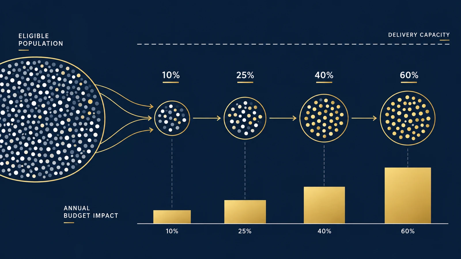
A new healthcare intervention has passed its economic evaluation. The clinical evidence is favorable. The incremental cost-effectiveness ratio is acceptable.
Should the health system immediately offer it to every eligible patient? Not necessarily.
Cost-effectiveness asks whether the additional health gained is worth the additional cost. Implementation creates another question: How much money will actually be required as patients begin receiving the intervention?
That question depends heavily on something that can look deceptively simple: uptake.
An intervention can represent good value per patient while creating substantial short-term expenditure if the eligible population is large or adoption happens quickly. That makes uptake more than a forecasting assumption. It can become a decision variable.
From Value to Implementation
Consider a hypothetical intervention with 100,000 eligible patients, $8,000 incremental treatment cost per patient, $1,500 expected healthcare cost offset per treated patient, and $6,500 net incremental cost per treated patient.
If every eligible patient were treated immediately:
But healthcare adoption rarely moves instantly from 0% to 100%.
| Year | Uptake | Treated patients |
|---|---|---|
| 1 | 10% | 10,000 |
| 2 | 25% | 25,000 |
| 3 | 40% | 40,000 |
| Year | Treated patients | Net cost per patient | Budget impact |
|---|---|---|---|
| 1 | 10,000 | $6,500 | $65.0M |
| 2 | 25,000 | $6,500 | $162.5M |
| 3 | 40,000 | $6,500 | $260.0M |
Three-year illustrative cumulative impact: $487.5 million.
Nothing about the intervention’s per-patient cost-effectiveness necessarily changed. What changed was how many patients received it and when. That is why affordability analysis needs a population model, not just an ICER.
Uptake Is Not the Same as Eligibility
One of the easiest modeling mistakes is to treat the eligible population as the treated population. Suppose 100,000 patients satisfy the clinical eligibility criteria. That does not mean 100,000 will receive treatment.
- Population
- Diagnosed
- Clinically eligible
- Accessible
- Offered
- Accept
- Initiate
- Remain on treatment
| Stage | Patients |
|---|---|
| Relevant population | 500,000 |
| Diagnosed | 300,000 |
| Clinically eligible | 120,000 |
| Accessible to participating providers | 100,000 |
| Offered treatment | 80,000 |
| Accept treatment | 68,000 |
| Initiate treatment | 60,000 |
A model that simply uses 120,000 eligible patients as the treated population could materially overstate near-term expenditure. The opposite can also happen. If diagnosis expands after a new intervention becomes available, the treated population may grow faster than historical utilization suggests.
Eligibility and uptake therefore need separate assumptions.
A Simple Uptake Equation
For a basic model:
This is intentionally simplified. Real models may need to account for incident versus prevalent patients, treatment discontinuation, mortality, switching, market share, multiple comparators, adverse-event costs, administration costs, delayed benefits, and capacity constraints.
But even the simple structure reveals something important: Budget impact is driven by both economics per patient and the number of patients moving through the system.
Worked Example: Fast Adoption vs. Phased Adoption
Suppose the same intervention has an eligible population of 100,000, net incremental treatment cost of $6,500 per patient, and implementation cost of $2 million per year.
Scenario A — Fast Adoption
Uptake is 20% in Year 1, 40% in Year 2, and 60% in Year 3.
Scenario B — Phased Adoption
Uptake is 10% in Year 1, 25% in Year 2, and 40% in Year 3.
| Year | Fast uptake | Fast BI | Phased uptake | Phased BI |
|---|---|---|---|---|
| 1 | 20% | $132.0M | 10% | $67.0M |
| 2 | 40% | $262.0M | 25% | $164.5M |
| 3 | 60% | $392.0M | 40% | $262.0M |
Three-year totals are $786.0 million for fast adoption and $493.5 million for phased adoption. The difference is $292.5 million.
The phased strategy therefore requires substantially less expenditure over this three-year window. But that does not prove phased adoption is better. Patients who receive treatment later may also receive health benefits later. Budget management and health maximization are not the same objective. A complete decision must consider both.
Delaying Spending Can Also Delay Health Benefits
Suppose treatment produces an expected health benefit of 0.40 incremental QALYs per treated patient. In this simplified example, cumulative patient-treatment counts over three years are 120,000 for fast adoption and 75,000 for phased adoption.
The difference is 45,000 treatment-period observations. If we apply the illustrative 0.40 QALY gain directly for demonstration:
The fast-adoption scenario is therefore associated with more health benefit during the modeled implementation window. This calculation is deliberately simplified and should not be interpreted as a real clinical estimate.
In a proper model, health outcomes would depend on treatment timing, duration, disease progression, mortality, discounting, and the underlying clinical evidence.
The point is conceptual: Reducing near-term budget impact by slowing adoption can create an opportunity cost in delayed health benefit. That trade-off should be explicit.
Uptake Can Be Modeled as a Curve
Adoption does not always increase linearly. A new technology might experience slow start → rapid expansion → saturation.
| Year | Uptake |
|---|---|
| 1 | 5% |
| 2 | 12% |
| 3 | 28% |
| 4 | 47% |
| 5 | 60% |
This can occur because clinicians need training, reimbursement expands gradually, provider capacity increases, awareness grows, evidence accumulates, supply improves, or patient acceptance changes. For some technologies, uptake may instead spike rapidly and then stabilize.
The model should therefore avoid assuming that uptake grows linearly merely because linear growth is easy to calculate.
Uptake Is Often One of the Largest Sources of Uncertainty
Recent budget-impact studies continue to show how sensitive affordability can be to adoption assumptions. For example, a 2026 ISPOR budget-impact analysis of biologic therapies for severe eosinophilic asthma reported that results were particularly sensitive to uptake rate, eligible population size, and drug acquisition cost.
Another 2026 analysis examining expanded Medicare coverage of GLP-1 therapies explicitly modeled uptake alongside alternative pricing scenarios when estimating pharmacy budget impact.
These examples do not establish universal uptake parameters. They illustrate why uptake should be tested rather than treated as a fixed certainty.
Build an Uptake Sensitivity Matrix
Suppose eligible population is 100,000 and cost offset is $1,500 per treated patient. Now vary both uptake and incremental treatment cost.
| Uptake | $6,000 treatment cost | $8,000 treatment cost | $10,000 treatment cost |
|---|---|---|---|
| 10% | $45M | $65M | $85M |
| 25% | $112.5M | $162.5M | $212.5M |
| 40% | $180M | $260M | $340M |
| 60% | $270M | $390M | $510M |
For example, at 40% uptake and $8,000 treatment cost:
This table reveals an important interaction. Price and uptake multiply. A 10% price reduction can matter; a 20-percentage-point uptake change can matter; their combined effect can be much larger than discussing either assumption in isolation.
The Eligible Population Also Deserves Sensitivity Analysis
Suppose the epidemiological estimate of 100,000 eligible patients is uncertain. Test low at 80,000, base at 100,000, and high at 130,000.
| Population | Calculation at 40% uptake and $6,500 net cost | Budget impact |
|---|---|---|
| Low: 80,000 | 80,000 × 40% × $6,500 | $208M |
| Base: 100,000 | 100,000 × 40% × $6,500 | $260M |
| High: 130,000 | 130,000 × 40% × $6,500 | $338M |
The difference between the low and high population assumptions is $130 million. This demonstrates why epidemiology is not merely background information in a budget-impact model. It can be one of the primary financial drivers.
Capacity Can Put a Ceiling on Uptake
Not every adoption curve is driven by demand. Suppose a therapy requires administration at specialized centers. The eligible population may support 40,000 patients in Year 1, but the delivery network can treat only 12,000.
Then: Clinical demand ≠ operational capacity
Suppose demand-based uptake predicts 20,000 patients and capacity is 12,000. Actual modeled treatment is 12,000. If net incremental cost is $6,500:
rather than:
The capacity constraint changes both expenditure and access. This is where budget-impact analysis begins to connect with operations research and implementation planning.
Market Share Can Matter Too
A new intervention may not simply add patients. It may replace existing treatments.
Suppose 50,000 patients are treated in a market with Current Therapy A at 60% and Current Therapy B at 40%. A new intervention enters and reaches 25% market share.
If total treatment volume remains unchanged, the budget question is not: What does treating 12,500 patients cost? It is: What is the incremental cost of moving 12,500 patients from the displaced treatment mix to the new intervention?
That requires a scenario without the new technology and a scenario with it. Budget impact is the difference between those scenarios.
Cost Offsets Need Timing
Suppose a treatment costs $8,000 more upfront but is expected to reduce hospitalizations by $3,000 per patient. It may be tempting to write:
But what if the $3,000 savings occurs gradually over three years? The first-year payer budget may still absorb most of the $8,000 acquisition cost before receiving the full downstream offset.
This is particularly important for interventions with high upfront acquisition costs, delayed complications avoided, long-term disease modification, or curative intent. Affordability depends not only on how much cost is offset but when.
Budget Impact Is Not ICER × Population
This deserves repeating.
The ICER is a ratio of incremental cost to incremental health effect. Budget impact requires actual population flows and costs.
The model instead needs quantities such as number eligible, number treated, current treatment cost, new treatment cost, market displacement, implementation cost, cost offsets, and uptake over time.
Cost-effectiveness and budget impact answer related but different questions. The existing cost-effectiveness versus budget impact analysis explores that distinction in more detail.
Use Scenario Analysis Before Claiming Affordability
A useful model might present at least three scenarios.
- Conservative Adoption — slower uptake, lower eligible population.
- Base Case — most plausible assumptions.
- Rapid Adoption — faster uptake, higher eligible population.
| Scenario | Eligible | Year-3 uptake | Year-3 treated | Net cost/patient | Year-3 BI |
|---|---|---|---|---|---|
| Conservative | 80,000 | 25% | 20,000 | $6,500 | $130M |
| Base | 100,000 | 40% | 40,000 | $6,500 | $260M |
| Rapid | 130,000 | 60% | 78,000 | $6,500 | $507M |
The range is large: $130 million to $507 million. That range is not a weakness of the model. If the underlying assumptions are genuinely uncertain, displaying that uncertainty is more informative than presenting a single precise-looking number.
Do Not Turn the Model Into a Forecast Claim
An uptake model is not automatically a forecast. If the model assumes 40% adoption in Year 3, that does not mean 40% adoption will occur.
It means: If uptake reaches 40%, given the other assumptions, this is the modeled financial consequence.
Observed historical uptake can inform the assumption. Expert opinion can inform it. Comparable launches can inform it. But those inputs do not make the scenario causally determined.
The model should clearly distinguish assumption from observed evidence from modeled consequence.
The Decision Is Bigger Than “Can We Afford It?”
A good implementation model can support several decisions:
- Can the payer absorb rapid adoption?
- Would phased implementation reduce near-term pressure?
- Which assumption creates the largest financial risk?
- Would a price agreement materially change affordability?
- Does provider capacity constrain adoption before the budget does?
- Which patient groups might reasonably be prioritized first?
These questions turn a static economic result into a decision model.
From Economic Evaluation to Implementation Strategy
- Clinical evidence
- Cost-effectiveness
- Eligible population
- Uptake scenarios
- Capacity
- Budget impact
- Uncertainty
- Implementation strategy
A health system does not make decisions with an ICER alone. It must translate evidence into populations, timelines, resources, and constraints.
That is why a technology can be clinically effective, cost-effective, and still require a carefully designed adoption strategy.
The purpose of budget-impact modeling is not to argue that expensive interventions should be delayed. It is to make the implementation consequences visible before the budget is committed.
The site’s decision-threshold framework provides a related way to connect evidence and uncertainty to action. For healthcare-specific analytical work, see the Health Economics & Outcomes Research service.
References / Further Reading
- NICE — Technology appraisal and highly specialised technologies guidance: the manual
- ISPOR — Principles of Good Practice for Budget Impact Analysis
- ISPOR Asia Pacific 2026 — Affordability of Biologic Add-On Therapy for Severe Eosinophilic Asthma in Thailand
- ISPOR 2026 — Expanded Medicare coverage of GLP-1 therapies and pharmacy budget impact
Does a Healthcare Intervention Make Sense Beyond the ICER?
UAD Consulting helps structure cost-effectiveness, budget-impact, simulation, and decision models so healthcare evidence can be translated into practical implementation and resource-allocation questions.
Explore ServicesGet in Touch