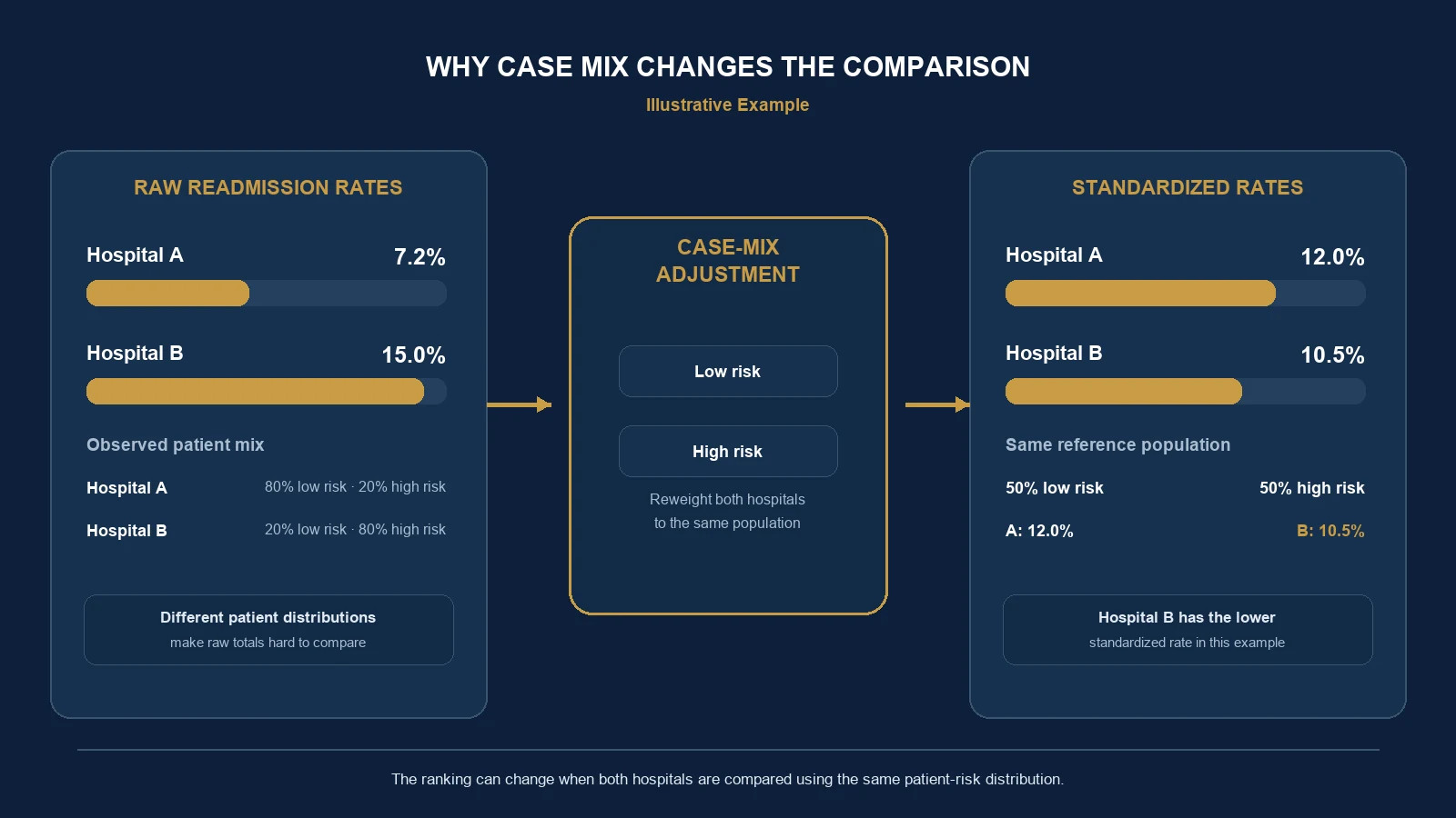
Imagine two hospitals being evaluated on their 30-day readmission rates.
Hospital A reports that 7.2% of its patients were readmitted.
Hospital B reports a substantially higher rate of 15.0%.
At first glance, Hospital A appears to perform much better.
A healthcare administrator might interpret this difference as evidence of stronger discharge planning, better care coordination, or more effective clinical management.
But there is an important question missing from that comparison:
Were the two hospitals treating patients with similar risks of readmission?
Suppose Hospital A primarily treats relatively low-risk patients, while Hospital B serves a much larger proportion of patients with complex medical conditions.
The difference in their overall readmission rates may reflect patient characteristics as well as differences in care.
In fact, it is possible for Hospital B to have lower readmission rates within every patient-risk group while still reporting a higher overall readmission rate.
This is not a contradiction.
It is a consequence of how different patient populations are combined.
Understanding this problem is essential for healthcare quality measurement, hospital benchmarking, outcomes research, and the interpretation of administrative healthcare data. AHRQ describes its Quality Indicators as standardized measures that can be applied to hospital administrative data, while also distinguishing measure purposes and populations [3].
What Is Risk Adjustment in Healthcare Analytics?
Risk adjustment is a statistical approach used to account for differences in patient characteristics that may influence healthcare outcomes.
The purpose is to make comparisons more meaningful when organizations treat populations with different underlying risks.
For example, the probability of hospital readmission may vary according to:
- Age
- Existing medical conditions
- Severity of illness
- Previous hospitalizations
- Functional limitations
- Relevant clinical history
- Other patient characteristics associated with readmission risk
Not every variable belongs in every risk-adjustment model. The appropriate factors depend on the outcome, population, available evidence, and purpose of the comparison.
A hospital treating a higher-risk population may have more readmissions even if its care processes are effective. Conversely, a hospital treating relatively healthy patients may have a low readmission rate without necessarily delivering superior care.
Risk adjustment attempts to separate differences in patient composition from differences in observed outcomes.
It does not eliminate every source of bias. Nor does it automatically establish that one hospital provides better care than another.
Why Raw Readmission Rates Can Be Misleading
A raw readmission rate is straightforward to calculate. For a defined cohort:
For example:
This calculation is useful. It describes the observed frequency of readmission within the defined population.
But the rate depends on more than the quality of care. It also depends on who was included in the denominator.
A hospital serving patients with substantial comorbidities may face a different baseline readmission risk than a hospital serving a healthier population. Comparing their raw rates without considering these differences can produce misleading conclusions.
Before interpreting a readmission rate, analysts should also establish the measure specification. For example:
- Does the measure include all-cause or condition-specific readmissions?
- Does it count planned readmissions?
- Which index admissions qualify?
- How are transfers handled?
- Can readmissions to another hospital be observed?
- What happens when a patient dies during follow-up?
- Are repeat admissions for the same patient eligible as separate index events?
These questions matter because different definitions can produce different rates.
For this article, the numerical example uses a simplified hypothetical measure of 30-day unplanned readmission after an eligible index discharge. It is not intended to reproduce a specific CMS quality measure.
A Worked Example: Two Hospitals, Two Patient-Risk Groups
Consider two hypothetical hospitals. Each hospital has 1,000 eligible index discharges. Patients are divided into two groups: low-risk patients and high-risk patients.
Assume these categories are determined using relevant patient characteristics available before the outcome occurs. Also assume that readmissions are captured consistently across both hospitals.
The observed data are:
| Hospital | Risk Group | Discharges | Readmissions | Readmission Rate |
|---|---|---|---|---|
| A | Low risk | 800 | 32 | 4.0% |
| A | High risk | 200 | 40 | 20.0% |
| B | Low risk | 200 | 6 | 3.0% |
| B | High risk | 800 | 144 | 18.0% |
These values are entirely hypothetical. They were constructed to demonstrate how patient composition can affect an aggregate comparison.
Step 1: Calculate the Overall Rate for Hospital A
Hospital A has 800 low-risk discharges and 200 high-risk discharges, for a total of 1,000. Readmissions are 32 + 40 = 72.
Hospital A's raw readmission rate = 7.2%
Step 2: Calculate the Overall Rate for Hospital B
Hospital B has 200 low-risk discharges and 800 high-risk discharges, for a total of 1,000. Readmissions are 6 + 144 = 150.
Hospital B's raw readmission rate = 15.0%
Step 3: Compare the Raw Results
| Hospital | Total Discharges | Readmissions | Raw Rate |
|---|---|---|---|
| A | 1,000 | 72 | 7.2% |
| B | 1,000 | 150 | 15.0% |
Hospital B's raw rate is 7.8 percentage points higher. A simple comparison suggests that Hospital A performs substantially better.
But look again at the original risk-group data. Among low-risk patients, Hospital A is at 4.0% and Hospital B at 3.0%. Among high-risk patients, Hospital A is at 20.0% and Hospital B at 18.0%.
Hospital B has a lower readmission rate in both groups. How can Hospital B perform better within each group but worse overall?
The answer is patient composition.
Simpson's Paradox: When the Aggregate Reverses the Subgroup Comparison
This example illustrates Simpson's paradox. Simpson's paradox occurs when a relationship observed within groups changes direction or disappears after those groups are combined.
In our example, Hospital B has lower readmission rates in both risk categories. Yet its overall readmission rate is higher.
The reason is that the hospitals treat very different patient populations.
- Hospital A's patient mix: 80% low risk and 20% high risk.
- Hospital B's patient mix: 20% low risk and 80% high risk.
High-risk patients have substantially higher readmission rates in both hospitals. Because Hospital B treats many more high-risk patients, those patients contribute much more heavily to its overall rate.
The aggregate comparison therefore combines two different elements:
- Readmission rates within patient-risk groups.
- The proportion of patients belonging to each group.
The raw rate does not distinguish between these effects. This is why hospital comparisons should begin with an examination of patient composition rather than assuming that an aggregate difference represents a difference in care quality.
How Direct Standardization Changes the Comparison
One way to make the comparison more meaningful is to calculate what each hospital's readmission rate would look like under the same patient-risk distribution.
This approach is called direct standardization. The method applies each hospital's observed risk-group-specific rates to a common reference population.
For our example, suppose the reference population contains 50% low-risk patients and 50% high-risk patients.
This reference distribution is chosen solely to illustrate the calculation. It is not an official CMS standard population. The CDC describes direct standardization as applying group-specific rates to a standard distribution and cautions that adjusted rates are relative indexes, not actual observed risks [2].
Standardized Rate Formula
For two risk groups:
+ (High-Risk Weight × High-Risk Readmission Rate)
The weights must sum to 1.
Here, the low-risk weight is 0.50 and the high-risk weight is 0.50.
Hospital A
Hospital A's observed rates are 4% for low-risk patients and 20% for high-risk patients.
= 2% + 10%
Hospital A standardized rate = 12.0%
Hospital B
Hospital B's observed rates are 3% for low-risk patients and 18% for high-risk patients.
= 1.5% + 9%
Hospital B standardized rate = 10.5%
Compare the Results
| Hospital | Raw Rate | Standardized Rate |
|---|---|---|
| A | 7.2% | 12.0% |
| B | 15.0% | 10.5% |
The ranking reverses. Using the raw rates, Hospital A appears better. Using the standardized rates, Hospital B has the lower readmission rate.
This is the central lesson of the example.
The same observed patient outcomes can support different aggregate comparisons depending on how patient composition is handled.
No patient's outcome changed. The analysis changed the population weights used for comparison.
Does This Prove Hospital B Provides Better Care?
No. Hospital B has the lower directly standardized readmission rate under the assumptions of this example. That is a descriptive statistical result.
It does not establish that Hospital B's care caused fewer readmissions. Several alternative explanations remain possible.
First, the two risk groups may be too broad. Patients classified as high risk may still differ substantially in disease severity, functional status, prior utilization, or other clinically relevant characteristics.
Second, important confounders may be unmeasured.
Third, readmission data may be incomplete.
Fourth, coding practices may differ across hospitals.
Finally, the standardized difference may reflect random variation. Hospital B's low-risk group contains only 200 discharges and six readmissions. Its estimated 3% rate is therefore based on relatively few events.
A rigorous analysis would quantify uncertainty rather than treating every observed percentage as equally precise.
Risk adjustment improves the structure of a comparison. It does not automatically establish a causal difference in healthcare quality.
Direct Standardization Is Not the Same as CMS Risk Standardization
The simplified calculation above is useful for explaining case-mix adjustment. However, official healthcare quality measurement can be considerably more sophisticated.
The Centers for Medicare & Medicaid Services uses risk-standardized readmission measures in its Hospital Readmissions Reduction Program (HRRP). CMS describes the excess readmission ratio as a comparison of predicted and expected unplanned readmissions and calculates an excess readmission ratio for each included condition or procedure [1].
It is not equivalent to applying two fixed weights to two patient-risk groups.
Another important distinction concerns the measures themselves. The HRRP includes selected condition- and procedure-specific measures. The Hospital-Wide All-Cause Readmission measure belongs to a separate quality-reporting context. CMS states that the hospital-wide measure is not included in the HRRP [1].
These measures should not be treated as interchangeable. A hospital's result for heart failure readmissions is not automatically the same as its hospital-wide readmission performance.
The population, exclusions, modeling approach, and reporting program must be identified before interpreting an official performance measure.
For formal benchmarking, analysts should follow the exact specifications for the applicable measure and reporting period.
The educational direct-standardization example in this article should not be substituted for official CMS calculations.
Why the Choice of Reference Population Matters
Direct standardization requires a reference population. In our example, we used 50% low risk and 50% high risk.
But suppose the reference population contained 80% low-risk patients and 20% high-risk patients.
Hospital B = (0.80 × 3%) + (0.20 × 18%) = 6.0%
Now suppose the reference population contained 20% low-risk patients and 80% high-risk patients.
Hospital B = (0.20 × 3%) + (0.80 × 18%) = 15.0%
| Reference Population | Hospital A | Hospital B |
|---|---|---|
| 80% low / 20% high | 7.2% | 6.0% |
| 50% low / 50% high | 12.0% | 10.5% |
| 20% low / 80% high | 16.8% | 15.0% |
Hospital B remains lower under all three reference distributions because its observed rate is lower in both risk groups. But the numerical difference changes.
This illustrates why a standardized rate should always identify the population used for standardization. The CDC describes direct age standardization using the same general weighted-average principle. Age-adjusted rates are useful comparative measures, but they should not be interpreted as the actual observed risk in a population [2]. The same conceptual caution applies to our simplified patient-risk standardization.
What If Risk Groups Are Not Enough?
Real healthcare populations cannot always be represented adequately by two categories.
A patient may have several interacting risk factors. For example, an older patient with heart failure, diabetes, chronic kidney disease, and multiple previous admissions may have a different expected readmission risk from another patient in the same broad high-risk category.
A more advanced model might estimate individual readmission probabilities using patient-level characteristics.
These probabilities can be used within a risk-adjustment framework. Depending on the objective, analysts may use logistic regression, hierarchical models, or other appropriately validated methods.
However, the model must be designed around the measurement question. A highly predictive model is not necessarily an appropriate hospital benchmarking model.
For example, including variables that reflect care delivered by the hospital may inadvertently adjust away differences that the quality measure is intended to evaluate.
Risk adjustment should generally focus on appropriate patient characteristics rather than automatically controlling for every variable associated with the outcome. Research has examined how adding clinical and social patient characteristics can affect hospital readmission comparisons and payment implications [4, 5].
The distinction between prediction and comparison is essential.
Observed, Expected, and Risk-Standardized Outcomes
Another useful concept is the difference between observed and expected readmissions.
Observed readmissions are the events actually recorded.
Expected readmissions represent the number or rate predicted under a specified reference model and patient population.
A simplified observed-to-expected ratio is:
Suppose a hospital has 90 observed readmissions and 100 expected readmissions.
Under the assumptions of the expected-value model, the hospital experienced 10% fewer readmissions than expected.
However, this simple ratio is not automatically equivalent to the official CMS excess readmission ratio. CMS methodology can use model-based predicted and expected outcomes, including hierarchical estimation. The exact calculation must follow the applicable measure specification.
An O/E ratio also depends on the validity of the expected-outcome model. If the model is poorly calibrated, the ratio can be misleading.
A comparison should therefore evaluate both the outcome and the model used to establish the benchmark.
Five Problems That Risk Adjustment Does Not Automatically Solve
1. Incomplete Readmission Capture
A patient may be discharged from Hospital A and readmitted to Hospital B. If the analytical dataset only captures encounters at the original hospital, the readmission may be missed. This can bias the measured outcome. Cross-hospital linkage and longitudinal patient identification may be necessary.
2. Differences in Coding Practices
Administrative healthcare data depend on diagnosis and procedure coding. Hospitals may differ in coding completeness or documentation practices. If recorded comorbidities influence estimated patient risk, inconsistent coding can affect adjusted comparisons. A diagnosis code is not always a complete representation of clinical severity.
3. Unmeasured Patient Characteristics
Risk adjustment can account only for characteristics that are measured and appropriately included. Important factors may be absent from the dataset. Examples can include functional status, clinical severity, access to follow-up care, and other contextual variables.
4. Statistical Uncertainty
A hospital with a small number of eligible discharges may have an unstable estimated readmission rate. A few additional events can materially change the result.
Confidence intervals, uncertainty estimates, and appropriate methods for low-volume hospitals should be considered. A ranking based on small numerical differences may not be statistically meaningful.
5. Social and Environmental Factors
Readmission risk may also be associated with circumstances beyond the hospital. Examples include:
- Housing instability
- Transportation barriers
- Access to outpatient care
- Medication affordability
- Social support
- Neighborhood-level disadvantage
Whether and how to incorporate social risk factors into performance adjustment is a methodological and policy question. There is no universal answer.
Adjustment may improve comparability, but it may also obscure disparities if applied without considering the purpose of the measure.
Published research has examined how social risk adjustment changes hospital readmission comparisons and payment penalties [4]. The implications depend on the model, population, and policy objective.
Why Risk Adjustment Requires a Clear Analytical Objective
Risk adjustment is not a single procedure that should be applied identically to every healthcare analysis.
Consider three questions.
Question A: Which hospital has the lowest observed readmission burden?
For this question, raw rates may be directly relevant.
Question B: Which hospital has lower readmission rates after accounting for differences in patient characteristics?
This question requires a risk-adjusted comparison.
Question C: Would implementing a new discharge intervention reduce readmissions?
This is a causal question. Risk adjustment alone does not answer it.
The third question may require an experimental or quasi-experimental evaluation.
The analytical method must match the question.
A risk-adjusted association should not be presented as proof that a hospital policy caused better outcomes. Likewise, a lower observed readmission rate should not automatically be attributed to better clinical management.
A Practical Framework for Comparing Hospital Outcomes
A defensible comparison can be organized into eight steps.
Step 1: Define the Outcome
Specify exactly what counts as a readmission. Identify the follow-up period, eligible index discharges, planned versus unplanned admissions, relevant exclusions, and cross-hospital readmission capture.
Step 2: Define the Population
Determine which patients and encounters belong in the comparison. Avoid combining populations with fundamentally different eligibility rules.
Step 3: Examine the Raw Data
Calculate observed rates. Inspect patient counts, event counts, missing values, hospital volumes, patient characteristics, and coding distributions.
Step 4: Examine Case Mix
Determine whether the hospitals serve comparable populations. Identify clinically relevant differences.
Step 5: Select an Adjustment Method
Choose a method appropriate to the outcome and available data. Options may include stratification, direct standardization, regression-based adjustment, or hierarchical modeling.
Do not choose a more complex method solely because it is available.
Step 6: Validate the Model
Evaluate model assumptions, calibration, missing-data handling, variable definitions, relevant subgroup performance, and sensitivity to alternative specifications.
Step 7: Quantify Uncertainty
Report appropriate uncertainty measures. Avoid treating small differences in estimated rates as definitive rankings.
Step 8: Interpret the Results Carefully
Explain what was observed, what was adjusted, which population was used, what assumptions were required, which limitations remain, and what conclusions are and are not supported.
These steps should be reproducible. The broader importance of validating analytical inputs is discussed in UAD Consulting's article on data quality checks for analytics pipelines.
What Should a Hospital Dashboard Display?
A healthcare quality dashboard should not necessarily display one readmission percentage without context. A more informative design could include:
| Measure | Purpose |
|---|---|
| Raw readmission rate | Describes observed burden |
| Risk-adjusted rate | Supports a more comparable benchmark |
| Eligible discharge count | Shows population size |
| Readmission count | Shows the underlying number of events |
| Patient case-mix distribution | Explains population differences |
| Confidence interval | Communicates statistical uncertainty |
| Time trend | Shows changes across reporting periods |
| Measure definition | Clarifies inclusion and exclusion rules |
Not every dashboard needs every measure on its first screen. But the information should be accessible when users investigate a result.
A hospital administrator should be able to move from an aggregate rate to the underlying population and methodological context.
This is consistent with the broader principle of building a KPI framework around business decisions.
The purpose of a dashboard is not simply to display a number. It is to support a defensible interpretation of that number.
When Does This Matter Beyond Hospital Readmissions?
Hospital Mortality
Hospitals treating more critically ill patients may have higher raw mortality rates. Meaningful comparisons require careful attention to patient risk and measure specifications.
Emergency Department Outcomes
Differences in patient acuity, referral patterns, and service availability may influence observed outcomes.
Healthcare Costs
A hospital serving patients with more complex conditions may have higher average costs. That does not automatically mean its operations are less efficient.
Treatment Comparisons
Patients receiving different treatments may differ systematically before treatment begins. Risk adjustment can help address measured differences, but observational treatment comparisons require additional causal assumptions.
Insurance and Population Health
Differences in age, morbidity, and utilization history can influence observed spending and outcomes.
The common problem is the same:
An aggregate difference may reflect both the outcome process and the composition of the population being measured.
What Hospital Leaders Should Take Away
Return to our original comparison.
- Hospital A raw readmission rate: 7.2%
- Hospital B raw readmission rate: 15.0%
A simple ranking favors Hospital A. But Hospital B treats a substantially larger proportion of high-risk patients.
Within both risk categories, Hospital B has lower observed readmission rates.
When both hospitals are evaluated using the same 50/50 patient-risk distribution:
- Hospital A: 12.0%
- Hospital B: 10.5%
The ranking reverses.
This example does not prove that Hospital B provides superior care. It demonstrates why the original raw comparison was insufficient to support that conclusion.
The appropriate next step is not necessarily to discard raw rates. It is to interpret raw rates alongside case mix, standardized estimates, uncertainty, and the limitations of the available data.
A fair healthcare comparison does not begin by asking which hospital has the lowest number. It begins by asking whether the numbers describe comparable patients, outcomes, and measurement conditions.
That distinction can change how healthcare organizations evaluate performance, identify improvement opportunities, and allocate resources. UAD Consulting's health economics and outcomes research work supports transparent analysis of healthcare utilization, outcomes, costs, and administrative data.
References and Further Reading
- Centers for Medicare & Medicaid Services. Hospital Readmissions Reduction Program. CMS program and measure overview.
- Centers for Disease Control and Prevention, National Center for Health Statistics. Health, United States: Age Adjustment. Updated September 16, 2026. CDC direct standardization explanation.
- Agency for Healthcare Research and Quality. AHRQ Quality Indicator Tools for Data Analytics. AHRQ quality indicators.
- Rogstad TL, Gupta S, Connolly J, Shrank WH, Roberts ET. (2022). Social Risk Adjustment in the Hospital Readmissions Reduction Program: A Systematic Review and Implications for Policy. Health Affairs, 41(9), 1307–1315. Health Affairs article.
- Roberts ET, Zaslavsky AM, McWilliams JM. (2018). Assessment of the Effect of Adjustment for Patient Characteristics on Hospital Readmission Rates: Implications for Pay for Performance. JAMA Internal Medicine, 178(11), 1498–1507. PubMed record.
Make Healthcare Comparisons More Meaningful
UAD Consulting helps organizations analyze healthcare utilization, outcomes, costs, and administrative data using transparent analytical methods. From cohort construction and risk adjustment to reporting and decision support, the goal is to make complex healthcare evidence easier to interpret and use.
Explore ServicesGet in Touch