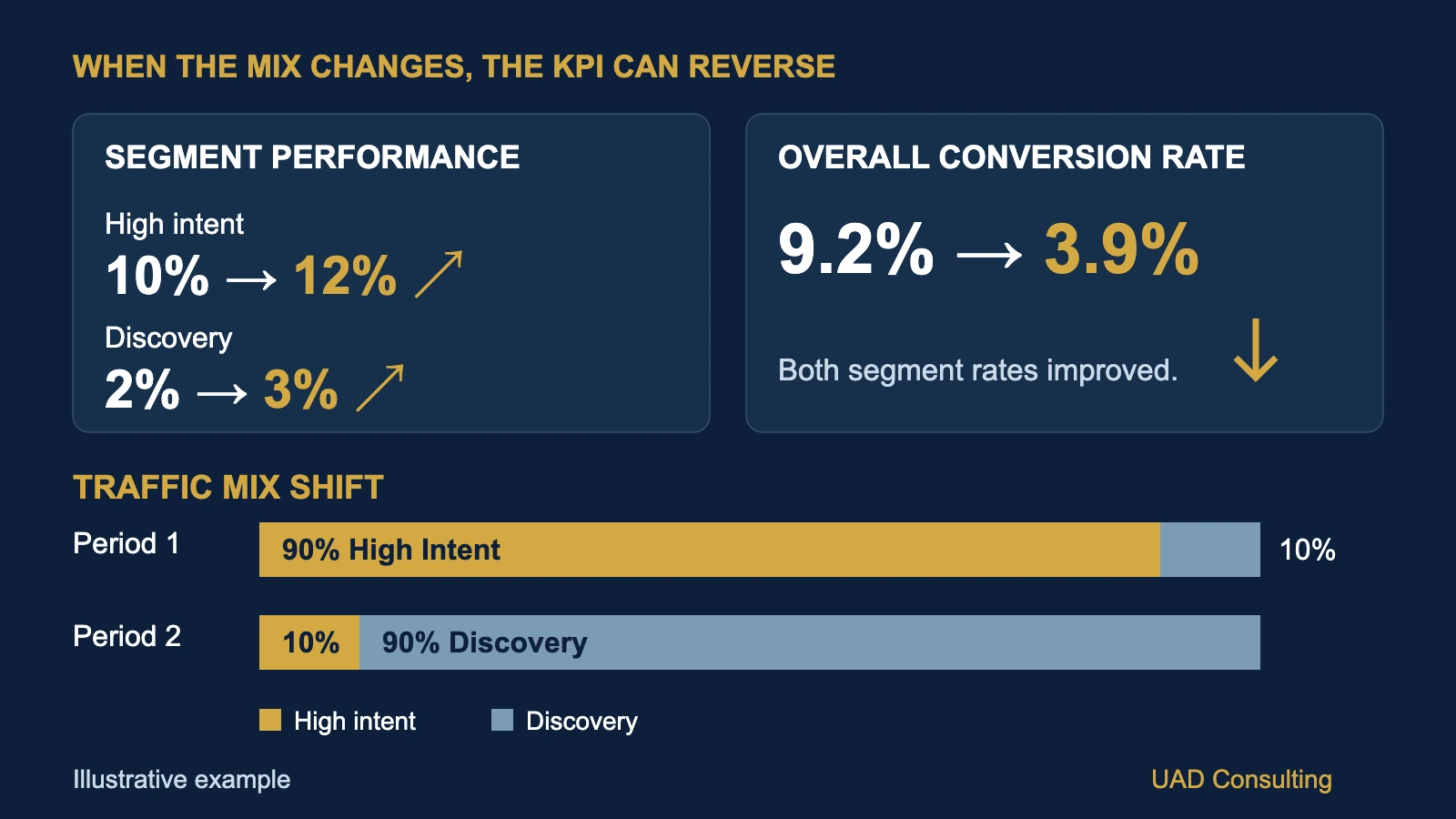
Your marketing dashboard shows that conversion rate declined from 9.2% to 3.9%.
That looks concerning.
Management wants to know what went wrong.
The marketing team investigates individual traffic segments and discovers something unexpected.
Conversion rates improved in every segment.
High-intent visitors converted more frequently.
Broader discovery traffic also converted more frequently.
Yet the overall conversion rate declined by more than half.
How can every segment improve while the total gets worse?
This is not necessarily a reporting error.
It can happen because the composition of the population being measured has changed.
The phenomenon is related to Simpson's paradox, a statistical pattern in which relationships observed within groups can reverse or disappear when those groups are combined.
For business analytics, this creates an important problem.
A dashboard can calculate every number correctly and still encourage the wrong interpretation.
Understanding why requires looking beyond the headline KPI.
The Short Answer: Your Traffic Mix May Have Changed
Overall conversion rate is a weighted average of the conversion rates of its component groups.
Each group's influence depends on how much of the total population it represents.
If a company receives more traffic from lower-converting segments, the overall conversion rate can decline even when conversion rates improve within every segment.
The reverse is also possible.
Overall conversion rate can increase while performance deteriorates within individual segments if the traffic mix shifts toward higher-converting groups.
This means an aggregate conversion rate combines two different phenomena:
- Changes in conversion performance within groups.
- Changes in the relative sizes of those groups.
A useful analysis separates these effects.
Otherwise, management may interpret a composition change as evidence that a website, campaign, or sales process became less effective.
The distinction is particularly important when budgets, acquisition strategies, or audience targeting change.
What Is Simpson's Paradox?
Simpson's paradox describes situations in which a relationship observed within separate groups differs from, disappears in, or reverses in the aggregated data.
The phenomenon is not limited to marketing.
It can appear in healthcare outcomes, educational statistics, operational performance, customer retention, financial analysis, and other settings involving grouped observations.
One historically influential example comes from research on graduate admissions at the University of California, Berkeley.
Bickel, Hammel, and O'Connell examined admissions data and showed how aggregate differences could be misleading when department-level application patterns were considered.
The original research was published in Science in 1975.
The general lesson is not that aggregated statistics are inherently wrong.
It is that the relationship between aggregation, group composition, and the underlying question matters.
A pooled statistic answers a question about the population as it is composed.
A segmented statistic answers a question about a particular subgroup.
Those questions are related but not interchangeable.
For business dashboards, the problem often appears when users compare overall performance across periods without considering changes in the population being measured.
A Worked Example: Two Traffic Segments
Consider a hypothetical company operating a lead-generation website.
The company divides website sessions into two mutually exclusive groups.
High-intent traffic includes sessions from visitors already searching for a specific solution or showing strong purchase intent.
Discovery traffic includes sessions from broader audiences who may still be researching their needs.
The business measures the percentage of sessions that generate at least one qualified lead.
For this example:
Sessions Generating a Qualified Lead
/
Total Sessions
Each session is counted once.
A session generating multiple qualified-lead events still counts as one converting session.
This distinction is important because event counts and converting-session counts are not necessarily identical.
The example uses hypothetical session-level data, not actual company performance.
Period 1: Before the Traffic Mix Changed
Suppose the website receives 1,000 sessions.
Of these:
900 sessions come from high-intent traffic.
100 sessions come from discovery traffic.
The results are:
| Segment | Sessions | Converting Sessions | Conversion Rate |
|---|---|---|---|
| High-intent traffic | 900 | 90 | 10.0% |
| Discovery traffic | 100 | 2 | 2.0% |
| Total | 1,000 | 92 | 9.2% |
The overall conversion rate is:
Most sessions belong to the higher-converting segment.
High-intent traffic represents 90% of total sessions.
Discovery traffic represents only 10%.
The overall rate therefore sits relatively close to the high-intent conversion rate.
Now suppose the company changes its acquisition strategy.
It begins reaching a much broader audience.
The composition of website traffic changes substantially.
Period 2: Every Segment Improves
During the second period, the website again receives 1,000 sessions.
However, the traffic mix is now very different.
Only 100 sessions come from high-intent traffic.
The remaining 900 sessions come from discovery traffic.
Meanwhile, conversion rates improve within both segments.
High-intent conversion rate increases from 10% to 12%.
Discovery conversion rate increases from 2% to 3%.
The results are:
| Segment | Sessions | Converting Sessions | Conversion Rate |
|---|---|---|---|
| High-intent traffic | 100 | 12 | 12.0% |
| Discovery traffic | 900 | 27 | 3.0% |
| Total | 1,000 | 39 | 3.9% |
The overall conversion rate is:
The aggregate KPI declined.
But neither segment's observed conversion rate declined.
Both improved.
Compare the Two Periods
| Metric | Period 1 | Period 2 | Change |
|---|---|---|---|
| High-intent conversion rate | 10.0% | 12.0% | +2.0 pp |
| Discovery conversion rate | 2.0% | 3.0% | +1.0 pp |
| High-intent traffic share | 90% | 10% | -80 pp |
| Discovery traffic share | 10% | 90% | +80 pp |
| Overall conversion rate | 9.2% | 3.9% | -5.3 pp |
"pp" means percentage points.
The overall conversion rate fell by 5.3 percentage points.
In relative terms:
A dashboard displaying only the overall conversion rate would show a substantial decline.
But the segmented data reveals a more complicated story.
The website is converting a greater proportion of sessions within each segment.
At the same time, the website is receiving far more sessions from the segment with a lower baseline conversion rate.
That composition change pulls down the aggregate.
Why Weighted Averages Explain the Result
An overall conversion rate is not the simple average of the segment conversion rates.
It is a weighted average.
The general formula is:
SUM(
Segment Traffic Share
×
Segment Conversion Rate
)
For Period 1:
High-intent share = 90%
High-intent conversion rate = 10%
Discovery share = 10%
Discovery conversion rate = 2%
Therefore:
(0.90 × 0.10)
+
(0.10 × 0.02)
For Period 2:
High-intent share = 10%
High-intent conversion rate = 12%
Discovery share = 90%
Discovery conversion rate = 3%
Therefore:
(0.10 × 0.12)
+
(0.90 × 0.03)
The arithmetic is correct.
The important change is the weight assigned to each segment.
The high-intent segment contributed 90% of traffic in Period 1.
It contributed only 10% in Period 2.
The overall metric changed partly because the business was measuring a different composition of sessions.
How to Separate Performance Change From Traffic Mix
Suppose management wants to understand whether conversion performance improved independently of the traffic composition change.
One useful descriptive method is direct standardization.
Instead of allowing segment weights to change between periods, evaluate both periods using the same reference weights.
For example, use Period 1's traffic composition as the reference population.
The fixed weights are:
High-intent traffic: 90%
Discovery traffic: 10%
Period 1's standardized conversion rate is:
+
(0.10 × 0.02)
Now apply those same weights to Period 2's segment rates.
(0.90 × 0.12)
+
(0.10 × 0.03)
The comparison becomes:
| Measure | Period 1 | Period 2 |
|---|---|---|
| Observed overall conversion rate | 9.2% | 3.9% |
| Conversion rate at Period 1 traffic mix | 9.2% | 11.1% |
The observed aggregate conversion rate declined.
But the standardized rate increased by 1.9 percentage points.
This does not mean the company actually achieved an 11.1% overall conversion rate in Period 2.
It did not.
The observed rate was 3.9%.
The standardized value answers a hypothetical descriptive question:
"What would Period 2's overall conversion rate have been if its segment rates were applied to Period 1's traffic mix?"
This comparison helps separate within-segment rate changes from population composition.
It is not a causal estimate of what would happen if management deliberately changed traffic allocation.
Decomposing the Overall KPI Change
The total observed change was:
We can separate this into two components using a sequential decomposition.
First, hold the original traffic mix constant and update the segment rates.
That produces the standardized Period 2 rate of 11.1%.
The within-segment rate component is:
Next, move from the original traffic mix to the actual Period 2 traffic mix while holding Period 2 segment rates fixed.
The composition component is:
Together:
+1.9 pp - 7.2 pp
This exactly reconciles the observed change.
| Component | Contribution |
|---|---|
| Within-segment rate change | +1.9 pp |
| Traffic composition change | -7.2 pp |
| Total observed change | -5.3 pp |
This is a descriptive accounting decomposition.
It is not a causal attribution of business outcomes.
The decomposition also depends on the chosen reference weights and the order in which changes are introduced.
Using Period 2 as the reference or using a symmetric decomposition can produce different component values while preserving the same total change.
For reporting, analysts should document the reference period and decomposition method.
The useful conclusion is not that traffic mix "caused" exactly 7.2 percentage points of the decline.
It is that the aggregate change can be mathematically reconciled through changes in segment rates and weights.
A Reproducible BigQuery SQL Example
The calculation can be implemented in SQL.
The following example uses GoogleSQL syntax for BigQuery.
It reproduces the hypothetical dataset directly inside the query.
No external dataset is required.
WITH segment_counts AS (

  SELECT *
  FROM UNNEST([

    STRUCT(
      'Before' AS period,
      'High intent' AS segment,
      900 AS sessions,
      90 AS converting_sessions
    ),

    STRUCT(
      'Before',
      'Discovery',
      100,
      2
    ),

    STRUCT(
      'After',
      'High intent',
      100,
      12
    ),

    STRUCT(
      'After',
      'Discovery',
      900,
      27
    )

  ])

),

segment_rates AS (

  SELECT
    period,
    segment,
    sessions,
    converting_sessions,

    SAFE_DIVIDE(
      converting_sessions,
      sessions
    ) AS conversion_rate

  FROM segment_counts

),

baseline_weights AS (

  SELECT
    segment,

    SAFE_DIVIDE(
      sessions,
      SUM(sessions) OVER ()
    ) AS baseline_weight

  FROM segment_rates

  WHERE period = 'Before'

)

SELECT

  r.period,

  SUM(r.sessions) AS sessions,

  SUM(r.converting_sessions)
    AS converting_sessions,

  ROUND(
    100 * SAFE_DIVIDE(
      SUM(r.converting_sessions),
      SUM(r.sessions)
    ),
    1
  ) AS observed_conversion_rate_pct,

  ROUND(
    100 * SUM(
      r.conversion_rate
      * w.baseline_weight
    ),
    1
  ) AS standardized_conversion_rate_pct

FROM segment_rates r

JOIN baseline_weights w
  USING (segment)

GROUP BY r.period

ORDER BY
  CASE r.period
    WHEN 'Before' THEN 1
    ELSE 2
  END;
Expected output:
| Period | Sessions | Converting Sessions | Observed Rate | Standardized Rate |
|---|---|---|---|---|
| Before | 1,000 | 92 | 9.2% | 9.2% |
| After | 1,000 | 39 | 3.9% | 11.1% |
The query demonstrates how aggregate and standardized conversion rates can be calculated from the same observations.
In production, additional validation is necessary.
The example assumes that the same two segments exist in both periods.
It also assumes that the segment definitions remain consistent.
If a segment is missing from one period, the analyst should not silently drop it from the calculation.
Doing so can invalidate the intended reference population.
Similarly, if a segment has zero sessions, its conversion rate is undefined.
The appropriate response depends on the analytical design and should not be replaced automatically with a zero conversion rate.
Why the Choice of Denominator Matters
Conversion rate calculations require a clearly defined unit of analysis.
Possible denominators include:
- Sessions
- Users
- Leads
- Qualified leads
- Opportunities
- Orders
- Eligible customers
These denominators answer different business questions.
For example:
Converting Sessions / Sessions
Converting Users / Users
Customers Acquired / Leads
These should not be combined casually.
A website can have multiple sessions from the same user.
A user can generate multiple events.
A lead may appear in several systems.
Google Analytics 4 distinguishes session key event rate from user key event rate.
The former measures the percentage of sessions with a key event.
The latter measures the percentage of users who trigger a key event.
Our worked example uses converting sessions.
It should not be interpreted as a user conversion rate or as the number of key events divided by sessions.
Before diagnosing a conversion rate decline, verify the denominator, event definition, identity rules, and analytical grain.
This connects to the broader problem of data grain and dashboard double-counting.
What Traffic Mix Changes Can Reveal
A changing traffic mix may reflect a real business decision.
For example, a company may intentionally expand into broader audiences to generate awareness and reach new customers.
Those audiences may convert at lower rates because they are earlier in the buying process.
In that situation, a lower aggregate conversion rate does not automatically mean the strategy failed.
The company may be trading immediate conversion efficiency for audience growth.
However, the opposite interpretation is also possible.
The new traffic may be low quality.
The campaign may be attracting visitors unlikely to become customers.
Or the company may be spending more without generating sufficient economic value.
Conversion rate alone cannot distinguish these possibilities.
Management should also evaluate downstream business outcomes.
Relevant measures may include:
- Qualified leads
- Sales opportunities
- Customer acquisition cost
- Revenue per session
- Customer lifetime value
- Contribution margin
- Acquisition payback
The appropriate measures depend on the business model.
A company should not conclude that lower conversion rates are acceptable merely because traffic volume increased.
It should evaluate whether the additional traffic creates sufficient business value.
Does Improving Conversion Rate Prove the Website Improved?
No.
In our hypothetical example, the observed conversion rate increased within both segments.
That is a descriptive result.
It does not establish why the rates increased.
Possible explanations include:
- Website improvements
- Changes in visitor intent
- Seasonal demand
- Different campaign targeting
- Pricing changes
- Product availability
- Random variation
- Changes in tracking
- Differences in customer composition
Even the labels "high intent" and "discovery" may contain heterogeneous subgroups.
The composition of visitors within each broad segment may also have changed.
Furthermore, the sample sizes in the example are relatively small.
The observed differences should not automatically be treated as statistically significant or stable.
A more complete analysis would examine uncertainty, repeatability, and alternative explanations.
If management wants to determine whether a website redesign caused conversion performance to improve, a credible experimental or causal evaluation may be necessary.
Standardization helps describe differences in observed composition.
It does not, by itself, identify the causal effect of a marketing or website intervention.
This distinction is consistent with the broader principle that theory and hypotheses matter in analytics.
How to Visualize Simpson's Paradox in a Dashboard
A dashboard should make composition changes visible rather than hiding them behind one aggregate KPI.
A practical design can use three connected views.
View 1: Overall Performance
Display the observed conversion rate for each period.
Period 1: 9.2%
Period 2: 3.9%
This answers:
"What happened to the overall KPI?"
The chart should show the numerator and denominator alongside the rate.
View 2: Segment Performance
Display the conversion rates of each segment across periods.
High intent:
Discovery:
This answers:
"How did observed performance change within each group?"
Use a consistent percentage scale to avoid exaggerating small differences.
View 3: Population Composition
Display the traffic share of each segment.
Period 1:
10% discovery
Period 2:
90% discovery
A 100% stacked bar chart can make the composition shift clear.
This answers:
"Did the population being measured change?"
Add a Standardized Comparison
Where appropriate, include a fourth diagnostic measure:
Conversion rate at fixed traffic mix.
Period 1: 9.2%
Period 2: 11.1%
Clearly label this as standardized rather than observed.
Do not display the standardized rate as though it were actual recorded business performance.
A good dashboard allows management to distinguish:
Observed aggregate change
Within-segment change
Population composition change
These views provide more useful context than an isolated conversion-rate trend.
For broader guidance, see UAD Consulting's KPI framework for business analytics.
A Practical Investigation Framework
When an overall business rate changes unexpectedly, a structured investigation can reduce the risk of premature conclusions.
Step 1: Validate the Metric
Confirm:
- Numerator definition
- Denominator definition
- Measurement period
- Time zone
- Data completeness
- Tracking consistency
- Duplicate handling
If the metric definition changed, historical comparisons may not be directly comparable.
Step 2: Identify Meaningful Segments
Possible dimensions include:
- Traffic source
- Customer type
- Device
- Geography
- Product
- Acquisition cohort
- Customer tenure
- Hospital or facility
- Operational workflow
Segments should correspond to meaningful business differences.
Avoid creating hundreds of arbitrary segments without a decision or hypothesis.
Step 3: Compare Segment Rates
Calculate the outcome rate for each segment and period.
Include numerators and denominators.
A percentage without its sample size can be misleading.
Step 4: Compare Segment Weights
Calculate each segment's share of the population.
Look for meaningful composition changes.
A stable aggregate can also conceal important shifts.
Step 5: Standardize When Appropriate
Choose a defensible reference population.
Calculate rates using consistent weights.
Document the choice of reference weights.
Ensure segments are comparable across periods.
Step 6: Evaluate Uncertainty
Assess whether observed changes are large enough to distinguish from ordinary sampling variation.
Consider confidence intervals or other appropriate uncertainty measures.
Avoid interpreting small differences as definitive improvements.
Step 7: Connect Results to Decisions
Ask what the analysis changes operationally.
Should management investigate tracking?
Review acquisition quality?
Evaluate campaign economics?
Improve a particular customer segment?
Run an experiment?
Or simply update the dashboard to provide better context?
The value of the analysis depends on the decision it supports.
When Should You Not Adjust for Segment Mix?
Standardization is useful, but it should not be applied automatically.
The correct analysis depends on the question.
If management wants to know the actual percentage of all website sessions that generated leads, the observed aggregate conversion rate is relevant.
That rate reflects the actual traffic composition.
If management wants to compare conversion performance under a common traffic composition, a standardized rate may be informative.
These are different estimands.
Neither should replace the other without considering the business question.
Segment selection also matters.
Adjusting for a variable that is itself affected by an intervention can change the meaning of the comparison.
In causal analysis, conditioning on certain variables can introduce rather than remove bias.
A standardized descriptive comparison should therefore not automatically be interpreted as an unbiased causal estimate.
The appropriate adjustment requires substantive knowledge of how the business process works.
Applications Beyond Marketing Analytics
The same issue can appear in other business functions.
Healthcare Analytics
A hospital network's overall readmission rate may change because the mix of patients or facilities changes.
Comparisons may require appropriate case-mix or risk adjustment.
However, descriptive standardization and formal risk-adjusted outcome modeling are not identical methods.
Operations Analytics
A manufacturing company may improve defect rates within each product line while overall defect rate increases because production shifts toward more complex products.
Customer Success
Retention may improve within subscription tiers while overall retention declines because the customer base shifts toward historically lower-retention tiers.
Sales Analytics
Close rates may improve within lead-quality groups while overall close rate declines as the company generates more early-stage or lower-intent opportunities.
Across these settings, the central question remains the same:
Did performance change within comparable groups, or did the composition of the measured population change?
Often, both occurred.
Frequently Asked Questions
Can overall conversion rate decrease while every segment improves?
Yes.
Overall conversion rate is a weighted average of segment conversion rates.
If the population shifts toward lower-converting segments, the aggregate can decline even when each segment's observed rate improves.
Is this always Simpson's paradox?
Not every change in a weighted average qualifies as a classic Simpson's paradox.
The term is most appropriate when aggregation creates a reversal or another important discrepancy relative to subgroup relationships.
A changing traffic mix is the underlying mechanism in this example.
Should I always report standardized conversion rates?
No.
Standardization is useful when the business question requires comparing rates under a common population composition.
Observed aggregate rates remain important because they describe actual overall performance.
Can traffic mix explain changes in customer acquisition cost?
Potentially.
If different audience segments have different conversion rates and acquisition costs, changes in their relative sizes can affect aggregate acquisition economics.
However, cost analysis also requires consistent spend and customer definitions.
Does a standardized conversion rate measure causal improvement?
No.
It is a descriptive comparison based on specified reference weights.
A causal claim requires additional assumptions and an appropriate evaluation design.
What should I do if the segment definitions changed?
First, establish comparable definitions.
If historical segments cannot be reconstructed consistently, avoid presenting the comparison as directly equivalent.
Document the limitation and consider alternative groupings or data sources.
The Dashboard Was Not Necessarily Wrong
Return to the original hypothetical company.
Its overall conversion rate declined from 9.2% to 3.9%.
Both traffic segments improved their observed conversion rates.
The difference arose because the traffic mix changed substantially.
Using the original traffic composition as a reference, the standardized conversion rate increased from 9.2% to 11.1%.
That does not erase the actual decline in overall conversion rate.
Nor does it prove that the website became more effective.
It provides a clearer description of the underlying measurements.
A strong analytics system should make these distinctions visible.
The objective is not to choose whichever metric tells the most favorable story.
It is to understand which question each metric answers.
Before concluding that performance improved or deteriorated, ask:
"Did the underlying rates change, did the population mix change, or did both change together?"
That question can prevent a mathematically correct dashboard from supporting a misleading business decision.
References and Further Reading
- Stanford Encyclopedia of Philosophy. Simpson's Paradox. A conceptual treatment of aggregation, subgroup relationships, and causal interpretation.
- Bickel, P. J., Hammel, E. A., and O'Connell, J. W. (1975). Sex Bias in Graduate Admissions: Data from Berkeley. Science, 187(4175), 398–404. DOI: 10.1126/science.187.4175.398.
- Google Analytics. Google Analytics Data API: Dimensions and Metrics. Official definitions of session key event rate and user key event rate.
All numerical values in the conversion-rate example are hypothetical.
They are not empirical estimates of a specific company's performance.
Build Dashboards That Explain Performance
UAD Consulting helps organizations connect business questions, data definitions, statistical analysis, and visualization to create more reliable decision-support systems.
Whether the challenge involves misleading aggregate metrics, marketing performance, customer segmentation, or executive reporting, the goal is to make the underlying evidence clearer and more useful.
Explore our BI & Data Visualization services to discuss a reporting or performance measurement challenge.
Explore ServicesGet in Touch