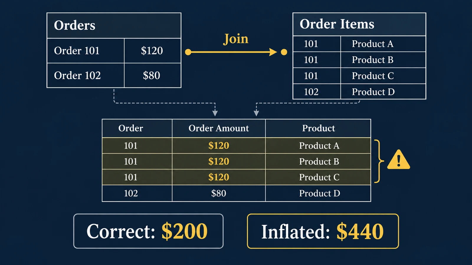
A dashboard can be technically correct and still report the wrong number.
The SQL may execute without errors. The joins may all be valid. The BI tool may faithfully sum the column it receives.
And yet revenue that should equal $200 appears as $440.
This often happens because the problem is not the calculation itself. It is the grain of the data being calculated.
Grain describes what one row in a dataset represents. One row might represent one customer, one order, one order line, one website session, one marketing campaign per day, one patient encounter, or one hospital per month.
Before combining tables or defining a metric, an analyst should be able to complete one sentence:
“One row in this table represents ______.”
If that sentence is unclear, aggregation errors become much more likely. This is especially important when dashboards combine operational, marketing, financial, or customer data at different levels of detail.
What Does Data Grain Mean?
Consider a simple orders table:
| order_id | customer_id | order_date | order_revenue |
|---|---|---|---|
| 101 | C01 | 2026-10-01 | $120 |
| 102 | C02 | 2026-10-01 | $80 |
The grain is one row per order. Total revenue is straightforward: $120 + $80 = $200.
Now consider an order-items table:
| order_id | product | quantity |
|---|---|---|
| 101 | Product A | 1 |
| 101 | Product B | 2 |
| 101 | Product C | 1 |
| 102 | Product D | 1 |
Its grain is different: one row per order line. Neither table is wrong. The problem begins when metrics from one grain are joined to another grain without accounting for the relationship.
How a Correct Join Creates the Wrong Total
Suppose we join the order-level revenue to the order-item table.
SELECT
    o.order_id,
    o.order_revenue,
    i.product,
    i.quantity
FROM orders o
JOIN order_items i
    ON o.order_id = i.order_id;
The result becomes:
| order_id | order_revenue | product |
|---|---|---|
| 101 | $120 | Product A |
| 101 | $120 | Product B |
| 101 | $120 | Product C |
| 102 | $80 | Product D |
The join is logically valid. Every item belongs to the correct order. But if a dashboard now calculates SUM(order_revenue), the result is $120 + $120 + $120 + $80 = $440.
Actual revenue is $200. The dashboard therefore overstates revenue by $440 − $200 = $240, or $240 / $200 = 120%.
Nothing about the SUM function is broken. The revenue measure was simply repeated at the lower order-line grain. This is why many dashboard discrepancies are data-modeling problems rather than visualization problems.
The Grain Test
Before joining two analytical tables, document three things for each table:
- What does one row represent?
- What columns uniquely identify that row?
- At what grain is each metric valid?
| Table | Grain | Unique Key | Example Metric |
|---|---|---|---|
| orders | One row per order | order_id | Order revenue |
| order_items | One row per order line | order_id + line_id | Item quantity |
| customers | One row per customer | customer_id | Signup date |
| daily_campaign | One row per campaign per day | campaign_id + date | Ad spend |
The grain contract is simple, but it prevents an important class of analytical errors.
Microsoft’s guidance for Power BI semantic models similarly emphasizes that fact tables should load data at a consistent grain and distinguishes dimension tables used for filtering and grouping from fact tables used for summarization. The underlying principle applies beyond any particular BI platform: know what a row represents before deciding what can safely be summed.
Why DISTINCT Is Usually Not the Real Fix
When analysts discover duplication, a common reaction is:
SUM(DISTINCT order_revenue)This can appear to solve the example above. It is not a reliable solution.
Suppose the two real orders were both worth $120:
| order_id | revenue |
|---|---|
| 101 | $120 |
| 102 | $120 |
Actual revenue is $240, but SUM(DISTINCT order_revenue) returns only $120 because DISTINCT operates on the value, not the business entity that generated it.
Similarly, SELECT DISTINCT * can sometimes hide duplicate rows without fixing the modeling logic that produced them.
The right question is not “How do I remove duplicates?” It is “At what grain should this metric be calculated?”
Four Common Ways Grain Breaks a Dashboard
1. One-to-Many Join Duplication
This is the order/order-item example. A metric stored once per parent entity is repeated across multiple child rows. Common examples include order revenue joined to order lines, customer attributes joined to sessions, invoices joined to invoice items, and patient encounters joined to diagnosis codes.
2. Many-to-Many Relationships
Suppose a campaign can belong to several audience groups and an audience group can contain several campaigns. Joining both directly can create combinations that multiply rows.
Many-to-many relationships are not inherently invalid, but they often require an explicit bridge table and a clearly defined allocation or measurement rule.
3. Mixing Snapshot and Transaction Data
Imagine a monthly customer snapshot:
| customer_id | month | account_balance |
|---|---|---|
| C01 | Jan | $1,000 |
| C01 | Feb | $1,200 |
| C01 | Mar | $1,100 |
The balance is a snapshot. Summing $1,000 + $1,200 + $1,100 = $3,300 usually does not mean the customer had $3,300 of economic activity. Some facts are additive across all dimensions; others are only additive across certain dimensions. A point-in-time balance is a classic example of a metric that requires different aggregation logic across time.
4. Combining Sources at Different Time Grains
Marketing data frequently creates this problem. Suppose ad spend is stored at campaign × date while conversions are stored at campaign × date × device.
Campaign A daily spend is $1,000:
| campaign | date | device | conversions |
|---|---|---|---|
| A | Oct 1 | Desktop | 12 |
| A | Oct 1 | Mobile | 18 |
| A | Oct 1 | Tablet | 2 |
After the join, the $1,000 spend may appear three times. A dashboard can then report $3,000 spend even though the source platform correctly reported $1,000.
This can easily be mistaken for a Google Ads, GA4, database, or BI-tool discrepancy when the real issue is grain mismatch.
Choose the Target Grain Before Writing the Join
A safer workflow is:
- Business Question
- Target Grain
- Source Grain
- Transformation
- Join
- Metric
Suppose the business asks, “What was revenue by product?” The target grain needs to support product. Order-level revenue cannot simply be repeated across products.
Depending on the data available, several valid approaches may exist. If line-level revenue is available, use it directly. If only order-level revenue exists, an allocation rule might be required. An order with $120 of revenue and three products could theoretically be allocated by item price, quantity, product list value, or another defensible business rule.
But the allocation rule becomes an analytical assumption and should be documented. It should not silently emerge from a join.
A Better SQL Pattern: Aggregate Before You Join
Sometimes the target analysis does not require lower-grain detail. Suppose you need order revenue and total item quantity per order. Instead of joining the raw line table, first aggregate the items to order grain.
WITH item_summary AS (
    SELECT
        order_id,
        SUM(quantity) AS total_quantity
    FROM order_items
    GROUP BY order_id
)

SELECT
    o.order_id,
    o.order_revenue,
    i.total_quantity
FROM orders o
LEFT JOIN item_summary i
    ON o.order_id = i.order_id;
Now both sides of the join represent one row per order.
This does not mean “always aggregate before joining.” Sometimes line-level analysis is exactly what the business needs. The principle is to transform the sources to a grain compatible with the analytical question before aggregating the metric.
A Pre-Join Cardinality Check
A useful diagnostic is to test whether the intended join key is actually unique.
SELECT
    order_id,
    COUNT(*) AS rows_per_order
FROM order_items
GROUP BY order_id
HAVING COUNT(*) > 1;
Finding multiple rows here is not necessarily an error. Order-items data is expected to contain multiple rows per order. But it tells the analyst that joining order-level measures onto this table will change the row count.
For a table that is supposed to contain one row per order, a stronger validation is:
SELECT
    COUNT(*) AS total_rows,
    COUNT(DISTINCT order_id) AS unique_orders
FROM orders;
If total_rows ≠ unique_orders, the assumed grain is already violated. This type of check belongs upstream in the analytical pipeline rather than being discovered after an executive notices that a dashboard total looks wrong.
Use data quality checks in analytics pipelines to extend this diagnostic into upstream completeness, uniqueness, validity, and reconciliation checks.
Row-Count Reconciliation Can Catch Join Explosions
Consider these counts:
| Pipeline Step | Rows | Intended Grain | Status |
|---|---|---|---|
| Orders | 100,000 | Order | Expected |
| + Customer | 100,000 | Order | Expected |
| + Order Items | 327,000 | Order line | Grain changed |
| Order aggregation | 100,000 | Order | Restored |
The increase from 100,000 to 327,000 may be completely legitimate if the resulting dataset intentionally operates at order-line grain. But if the analyst still believes the dataset represents one row per order, the increase is a warning.
The point is not that row counts must stay constant. The point is that changes in grain should be intentional and visible.
Star Schemas Help Make Grain Explicit
Dimensional models often separate facts from dimensions. A sales fact table might contain one row per order line, while dimensions provide descriptive context such as customer, product, geography, channel, and date.
Microsoft describes star-schema design as particularly relevant to semantic models because dimensions support filtering and grouping while facts support summarization. Kimball dimensional modeling likewise treats declaring the grain as a foundational design decision.
A simplified structure might be:
                 DimCustomer
                      |
    DimDate —— FactSales —— DimProduct
                      |
                  DimChannel
The important design question is not whether a model visually resembles a star. It is whether the fact table has a clearly declared and consistently enforced grain.
But Star Schema Is Not a Universal Performance Rule
Data modeling choices also depend on the analytical platform. For example, Google BigQuery supports nested and repeated fields and recommends denormalization with these structures for some hierarchical analytical workloads because it can reduce communication and join overhead.
Google also notes that star schemas are already optimized analytical structures in many situations, so further denormalization does not necessarily improve performance.
Logical correctness and physical optimization are related but different questions. A model can have a clearly defined business grain while being physically represented differently across a relational warehouse, BigQuery, a Power BI semantic model, or another analytical platform.
The goal is not to enforce one schema pattern everywhere. The goal is to preserve the meaning of the metrics.
Grain Problems Also Affect Ratios
Duplication does not only inflate totals. It can distort ratios.
Suppose actual revenue is $200 and actual marketing spend is $100. ROAS is $200 / $100 = 2.0.
If a join duplicates revenue to $440 but spend remains $100, reported ROAS is $440 / $100 = 4.4.
The dashboard now suggests marketing efficiency more than doubled. Nothing about campaign performance changed. The numerator and denominator were simply calculated at incompatible grains.
This is particularly dangerous because ratios often look plausible even when their components are wrong. See why dashboard numbers do not match for a related reconciliation perspective.
Grain Should Be Part of the Metric Definition
A strong metric contract should specify more than a formula.
| Field | Definition |
|---|---|
| Metric | Net Revenue |
| Business definition | Recognized order revenue after refunds and discounts |
| Source | Order financials |
| Base grain | One row per order |
| Aggregation | Additive across orders and selected reporting periods |
| Valid dimensions | Order date, customer, region |
| Special rule | Product reporting requires line-level revenue rather than repeating order-level revenue |
This is much safer than documenting only Net Revenue = SUM(net_revenue). The SQL formula is the final step. The grain determines whether that formula means what the business thinks it means.
A Practical Five-Step Grain Audit
When a dashboard total appears suspicious, use this sequence.
- State the expected grain. Write down what one row should represent in the final analytical dataset.
- Test uniqueness. Check whether the intended business key is actually unique.
- Measure row counts before and after joins. Identify exactly where the dataset expands or contracts.
- Reconcile a small known sample. Choose several orders, customers, campaigns, or encounters and manually trace them through the transformation.
- Validate metric aggregation. Confirm that each metric is being aggregated at a grain where its value is valid.
This sequence is usually more informative than randomly changing joins or adding DISTINCT until the dashboard total happens to look correct.
Does Double-Counting Prove the Join Caused the Business Change?
No. This distinction matters when dashboard errors are discovered during performance analysis.
Suppose reported revenue growth disappears after a grain problem is fixed. That demonstrates that the previous reporting calculation was inflated. It does not necessarily explain why underlying business performance changed.
Similarly, an observed relationship between customer type and revenue does not establish that customer type caused the revenue difference.
Data modeling determines whether the measurement is internally coherent. Causal inference answers a different question: “What would have happened under a different action or condition?” Correct measurement is necessary for causal analysis, but correct measurement alone does not establish causality.
The Most Important Question Before SUM()
Modern analytics tools make aggregation easy. That convenience can hide a fundamental modeling decision.
Before writing:
SUM(revenue)ask: revenue at what grain?
Before joining two tables, ask: what does one row represent on each side?
Before trusting a dashboard, ask: did the grain change anywhere between the source and the visualization?
These questions are simple. They are also among the most effective ways to prevent dashboards from confidently reporting the wrong answer.
- Business Question
- Grain
- Data Model
- Validation
- Metric
- Dashboard
- Decision
The dashboard is the visible end of the process. The reliability of the number is determined much earlier.
References / Further Reading
Build Dashboards on Metrics You Can Trust
UAD Consulting helps businesses structure analytical data, validate metrics, and build reporting systems that connect reliable data models with practical business decisions.
Explore ServicesGet in Touch