A subscription company launches a new customer onboarding process.
Management wants to evaluate whether customers are remaining active longer.
The analytics team creates a dashboard showing 90-day customer retention.
The result looks encouraging.
Of ten customers in a recent group, six have not canceled their subscriptions.
The dashboard reports:
Customer Retention = 6 / 10 = 60%.
But there is a problem.
Some customers joined only a few weeks ago.
They have not yet had the opportunity to complete a full 90-day observation period.
A customer who joined 25 days ago and remains active today is not necessarily a customer who will remain active for 90 days.
The dashboard may be treating incomplete observations as completed outcomes.
This creates a measurement problem known as right-censoring.
Right-censoring occurs when the event of interest has not been observed by the end of a customer's available follow-up period.
The customer may eventually cancel.
Or the customer may remain active for years.
At the reporting cutoff, the analyst simply does not know.
This distinction matters whenever businesses measure outcomes over time.
Examples include:
Customer churn.
Subscription duration.
Time to first purchase.
Time to repeat purchase.
Time to product adoption.
Time until account inactivity.
Time until equipment failure.
Time until a patient experiences a clinical event.
Traditional retention percentages can be useful when every customer has completed the required observation window.
When observation periods differ, survival analysis may provide a more appropriate framework.
One widely used method is the Kaplan–Meier estimator.
The Short Answer: Incomplete Follow-Up Is Not the Same as Retention
Suppose a company wants to estimate the probability that a customer remains subscribed through day 90.
For a customer who joined 120 days ago, the company can usually determine whether that customer remained subscribed through the first 90 days.
For a customer who joined only 30 days ago, the company cannot yet observe the complete 90-day outcome.
If the newer customer remains active, that tells us something useful.
The customer survived without cancellation through day 30.
But it does not establish survival through day 90.
The customer is right-censored at day 30.
A naive calculation may incorrectly count that customer as retained at day 90.
Alternatively, an analyst might exclude every customer without 90 days of follow-up.
That approach avoids treating incomplete observations as completed outcomes, but it discards available information and can change which customer cohorts are represented.
Survival analysis provides another option.
It uses the observed time until cancellation or censoring.
Under appropriate assumptions, it estimates the probability of remaining event-free over time.
For customer churn, the survival function can be interpreted as:
S(t) = P(Customer has not churned by time t)
The exact interpretation depends on how churn and the start of observation are defined.
The Kaplan–Meier estimator uses observed cancellations and the number of customers still at risk at each event time.
It does not treat censored customers as cancellations.
It also does not automatically treat them as having completed the full retention period.
What Is Right-Censoring?
Right-censoring means that an observation ends before the event of interest is observed.
Consider a customer who subscribes on September 1.
The company evaluates its data on September 30.
The customer remains subscribed.
The company has observed approximately 29 days without cancellation.
It does not know the customer's eventual cancellation date.
The customer is therefore right-censored at the end of available follow-up.
Now consider another customer.
This customer subscribes on January 1 and cancels on February 10.
The cancellation is observed.
The company knows the time from subscription to cancellation.
That observation is an event rather than a censored observation.
A time-to-event dataset therefore needs at least two important variables.
First:
Observed duration.
Second:
Event indicator.
The event indicator identifies whether the event actually occurred during observation.
A typical structure is:
event_observed = 1
when cancellation occurred.
event_observed = 0
when the customer was right-censored.
The distinction is essential.
A customer with event_observed = 0 is not necessarily a permanently retained customer.
The company simply did not observe cancellation during the available follow-up period.
A Worked Example: Ten Customers With Different Follow-Up Periods
Consider a hypothetical subscription company.
Ten customers entered the business at different calendar dates.
The company wants to estimate customer retention through day 90 after subscription.
Some customers canceled.
Others remained active until their available observation period ended.
The following table summarizes the data.
| Customer | Observed Days | Status |
|---|---|---|
| A | 15 | Canceled |
| B | 25 | Censored |
| C | 35 | Canceled |
| D | 45 | Censored |
| E | 55 | Canceled |
| F | 65 | Censored |
| G | 75 | Canceled |
| H | 90 | Censored |
| I | 90 | Censored |
| J | 90 | Censored |
All values are hypothetical.
They are not actual UAD Consulting client data.
Assume each customer is observed from the beginning of their subscription.
For simplicity, assume cancellation is the first qualifying subscription termination.
Also assume that customers B, D, and F are censored because the reporting cutoff occurs before they complete 90 days of follow-up.
Customers H, I, and J complete 90 days without an observed cancellation.
The dataset contains:
Ten customers.
Four observed cancellations.
Six observations without cancellation.
However, three of those six observations ended before day 90.
This distinction changes how the data should be interpreted.
Step 1: Calculate the Naive Retention Percentage
A simple dashboard might calculate:
Customers Without Observed Cancellation / Total Customers
There are six customers without observed cancellation.
There are ten customers overall.
Therefore:
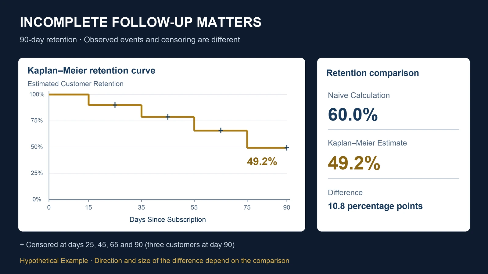
6 / 10 = 60%.
The dashboard reports 60% retention.
But what exactly does that number represent?
It represents the percentage of customers who had not canceled by their individual observation endpoints.
Those endpoints differ.
Some customers were observed for only 25 days.
Others were observed for 90 days.
The 60% figure therefore does not represent a consistently measured 90-day retention outcome.
It combines customers with different follow-up durations.
The arithmetic is correct.
The interpretation is not.
Step 2: Identify the Customers Still at Risk
The Kaplan–Meier estimator evaluates the number of customers still at risk immediately before each observed cancellation time.
A customer is at risk when the customer has not previously canceled and has not already been censored.
At the beginning:
Ten customers are at risk.
Customer A cancels on day 15.
Immediately before that cancellation:
Ten customers are at risk.
The conditional probability of remaining subscribed through the event time is estimated as:
1 - 1/10 = 0.90.
Estimated survival after day 15:
90%.
Customer B is censored on day 25.
This does not create a cancellation event.
The estimated survival curve does not decline at day 25.
However, Customer B no longer contributes to the risk set after day 25.
That matters when the next cancellation occurs.
Step 3: Apply the Kaplan–Meier Formula
The Kaplan–Meier estimator is commonly written as:
S(t) = Product over event times up to t of:
(1 - d_i / n_i)
Where:
S(t) = Estimated probability of remaining event-free through time t.
d_i = Number of observed events at event time i.
n_i = Number of individuals at risk immediately before event time i.
The estimator multiplies conditional survival probabilities across observed event times.
Censored observations remain in the risk set until their censoring times.
They are then removed from later risk sets.
Censoring does not directly lower the estimated survival curve.
Only observed events do.
For this example, cancellations occur on:
Day 15.
Day 35.
Day 55.
Day 75.
We can calculate the survival estimate at each event.
Step 4: Calculate Survival at Day 15
Ten customers are initially at risk.
One customer cancels.
The conditional survival factor is:
1 - 1/10 = 0.90.
Therefore:
S(15) = 0.90.
Estimated retention through day 15:
90%.
Customer B is censored at day 25.
The survival estimate remains 90%.
However, the risk set decreases by one.
Step 5: Calculate Survival at Day 35
Customer A already canceled.
Customer B was censored.
Therefore, eight customers remain at risk immediately before day 35.
Customer C cancels.
The conditional survival factor is:
1 - 1/8 = 7/8.
The cumulative survival estimate becomes:
S(35) = 0.90 × 7/8.
S(35) = 0.7875.
Estimated retention through day 35:
78.75%.
Customer D is censored at day 45.
Again, the survival estimate does not decline.
But the customer leaves the risk set for subsequent event times.
Step 6: Calculate Survival at Day 55
Six customers remain at risk immediately before day 55.
Customer E cancels.
The conditional survival factor is:
1 - 1/6 = 5/6.
The cumulative estimate becomes:
S(55) = 0.7875 × 5/6.
S(55) = 0.65625.
Estimated retention through day 55:
65.625%.
Customer F is censored at day 65.
The estimated survival probability remains unchanged at that time.
Step 7: Calculate Survival at Day 75
Four customers remain at risk immediately before day 75.
Customer G cancels.
The conditional survival factor is:
1 - 1/4 = 3/4.
The cumulative survival estimate becomes:
S(75) = 0.65625 × 3/4.
S(75) = 0.4921875.
Estimated retention through day 75:
49.21875%.
There are no additional observed cancellations before or on day 90.
Customers H, I, and J complete 90 days without cancellation and are administratively censored at that endpoint.
Therefore, the Kaplan–Meier estimate remains:
S(90) = 0.4921875.
Estimated 90-day retention:
Approximately 49.2%.
This estimate depends on the assumptions required for Kaplan–Meier analysis.
It is not the fully observed 90-day outcome for every individual customer.
Compare the Results
The completed calculation is:
| Event Day | Customers at Risk | Cancellations | Estimated Survival |
|---|---|---|---|
| 0 | 10 | 0 | 100.00% |
| 15 | 10 | 1 | 90.00% |
| 35 | 8 | 1 | 78.75% |
| 55 | 6 | 1 | 65.63% |
| 75 | 4 | 1 | 49.22% |
| 90 | 3 | 0 | 49.22% |
Censoring occurs on days 25, 45, 65, and 90.
The day-90 row shows the estimated survival probability before the three remaining customers are administratively censored at the analysis endpoint.
The resulting comparison is:
Naive percentage without observed cancellation:
60.0%.
Kaplan–Meier estimated 90-day retention:
49.2%.
Difference:
60.0% - 49.21875% = 10.78125 percentage points.
Approximately:
10.8 percentage points.
The naive calculation is higher in this hypothetical dataset.
However, this direction is not a universal property of every incomplete dataset.
Different censoring patterns, customer populations, and analytical definitions can produce different discrepancies.
The central issue is not that Kaplan–Meier always produces a lower retention estimate.
It is that incomplete observations must be handled according to what is actually known.
Why Does Censoring Change the Calculation?
The Kaplan–Meier estimator uses information from customers until the point when they leave observation.
Consider Customer B.
The company knows Customer B remained subscribed for 25 days.
That information contributes to estimating retention during the first 25 days.
But the company has no information about Customer B's subscription status after day 25.
Counting Customer B as retained through day 90 would assume an outcome that was never observed.
Counting Customer B as canceled at day 25 would also be incorrect.
Kaplan–Meier takes a different approach.
Customer B contributes to the risk set through the observed follow-up period.
After censoring, Customer B no longer contributes to subsequent risk sets.
This allows the estimator to use partial follow-up information without inventing an eventual event time.
However, the method relies on assumptions about the censoring process.
Those assumptions deserve careful attention.
The Critical Assumption: Non-Informative Censoring
Kaplan–Meier estimation commonly assumes that censoring is non-informative for the survival outcome.
In practical terms, customers who are censored should not have systematically different future cancellation risks from otherwise comparable customers who remain under observation.
Consider two situations.
Situation A: Administrative Censoring
A customer joins recently.
The reporting period ends before the customer reaches day 90.
The customer is censored because the company has not yet observed enough calendar time.
This is a common form of administrative censoring.
It may be reasonable to treat this censoring as non-informative under appropriate study conditions.
However, staggered customer acquisition can introduce additional complications.
For example, newer customers may have joined during a different marketing campaign or economic environment.
If cancellation risk changes across calendar cohorts, the censoring process may be associated with underlying retention differences.
Administrative censoring is not automatically harmless.
Situation B: Informative Loss of Observation
Suppose customers who experience billing problems are more likely to disappear from the company's tracking system.
Those same customers may also have higher cancellation risk.
The probability of being censored is now related to the outcome being studied.
The Kaplan–Meier estimator may be biased if this relationship is ignored.
A company should therefore distinguish:
Administrative end-of-study censoring.
Tracking failures.
Customer migration between systems.
Incomplete billing records.
Account merges.
Unknown subscription status.
These mechanisms are not necessarily equivalent.
The data collection process must be understood before interpreting the survival curve.
Reproduce the Calculation in Python
The following example uses Python's standard library.
No external packages are required.
Each observation contains:
Observed duration.
Event indicator.
The event indicator equals 1 for cancellation and 0 for censoring.
customers = [
    (15, 1),
    (25, 0),
    (35, 1),
    (45, 0),
    (55, 1),
    (65, 0),
    (75, 1),
    (90, 0),
    (90, 0),
    (90, 0),
]

horizon = 90

survival = 1.0

event_times = sorted({
    duration
    for duration, event in customers
    if event == 1 and duration <= horizon
})

results = []

for time in event_times:

    at_risk = sum(
        duration >= time
        for duration, event in customers
    )

    events = sum(
        duration == time and event == 1
        for duration, event in customers
    )

    survival *= (
        1 - events / at_risk
    )

    results.append({
        "day": time,
        "at_risk": at_risk,
        "events": events,
        "survival": survival
    })

for row in results:
    print(row)

print(
    "Estimated 90-day retention:",
    round(survival * 100, 4),
    "%"
)

assert abs(
    survival - 0.4921875
) < 1e-10
Expected result:
Estimated 90-day retention: 49.2188 %
The calculation is intentionally transparent.
It demonstrates the Kaplan–Meier product-limit estimator for a simple right-censored dataset.
It is not a complete production survival-analysis system.
A production implementation should handle additional issues such as:
Tied events.
Delayed entry.
Multiple customer subscription spells.
Time-dependent variables.
Competing events.
Uncertainty intervals.
Data-quality validation.
More complex applications may use specialized statistical software.
For example, the Python lifelines package provides a KaplanMeierFitter implementation with survival curves and confidence intervals.
Its official documentation is included in the references.
How Should the Dataset Be Built?
The statistical method is only as reliable as the underlying customer history.
A business should begin by defining the observation unit.
For example:
One customer.
One subscription.
One customer-product relationship.
One continuous subscription spell.
These are not interchangeable.
Suppose a customer subscribes to three products.
If the dataset contains one row per product subscription, the customer may appear three times.
That may be appropriate for product-level subscription analysis.
It may be inappropriate for customer-level retention.
The analyst should explicitly define the unit being followed.
A useful survival-analysis dataset can include:
| Field | Purpose |
|---|---|
| customer_id | Stable customer identifier |
| subscription_start | Beginning of follow-up |
| cancellation_date | Observed qualifying cancellation |
| observation_end | Last date with reliable status |
| duration_days | Observed time to event or censoring |
| event_observed | 1 for event, 0 for censoring |
| acquisition_cohort | Customer acquisition period |
| acquisition_channel | Source of customer acquisition |
| plan_type | Subscription category |
| reporting_cutoff | Date through which data are available |
The duration should be measured from a consistent time origin.
For example:
Subscription activation.
First paid subscription.
First successful transaction.
The correct starting point depends on the business question.
If some customers begin follow-up at account creation and others at first payment, their measured durations may not be comparable.
Customer Retention Is Not the Same as Revenue Retention
Survival analysis can estimate the probability that a customer remains subscribed over time.
It does not automatically measure how much revenue the company retains.
Suppose a company has two customers.
Customer A pays $100 per month.
Customer B pays $10,000 per month.
If Customer A cancels, the company loses one customer.
If Customer B cancels, the company also loses one customer.
In a simple customer-count survival analysis, both events count equally.
But their revenue consequences differ substantially.
This is why businesses should distinguish customer retention from revenue retention.
Customer survival analysis focuses on the timing of customer-level events.
Net revenue retention measures changes in recurring revenue from an existing customer cohort, including expansion, contraction, and churn.
These metrics answer different questions.
For a detailed explanation, see:
Revenue Is Growing. Why Are We Still Losing Customers?
The two approaches can complement each other.
A company may use survival analysis to understand when customers leave.
It may use revenue-retention metrics to understand the financial consequences of those departures.
Neither should automatically substitute for the other.
Can Survival Analysis Compare Different Customer Cohorts?
Yes.
Suppose a company introduces a new onboarding experience.
It wants to compare customers acquired before and after implementation.
A survival analysis can estimate retention curves for each group.
For example:
Historical onboarding cohort.
New onboarding cohort.
The curves may reveal differences in the timing of cancellations.
One group may experience more cancellations during the first 30 days.
Another may experience fewer early cancellations but more cancellations later.
A single 90-day retention percentage can conceal these patterns.
However, comparing survival curves does not automatically establish that the onboarding change caused the difference.
The cohorts may differ in:
Customer acquisition channels.
Pricing.
Customer demographics.
Subscription plans.
Market conditions.
Product features.
Promotional activity.
Calendar time.
These differences can influence retention independently of onboarding.
Survival analysis addresses time-to-event measurement and censoring.
It does not automatically eliminate confounding.
A causal evaluation of onboarding effectiveness requires an appropriate research design.
That may involve randomized assignment or a credible observational causal-inference approach.
The distinction is essential.
A difference between survival curves is an observed association.
It is not automatically an intervention effect.
Why Calendar Time Matters
A company may acquire customers continuously.
Some joined in January.
Others joined in September.
If retention is evaluated in October, the January customers have much longer potential follow-up.
The September customers may have only a few weeks of observation.
This is a natural setting for right-censoring.
However, customer behavior may also change over calendar time.
For example:
A pricing change may occur in June.
A new competitor may enter in August.
The company may introduce a different subscription plan in September.
The acquisition mix may change during the year.
If newer customers systematically differ from older customers, pooling all observations into one survival curve can obscure meaningful cohort differences.
A useful analysis may therefore estimate separate curves by acquisition cohort or use an appropriate survival regression model.
But segmenting the data creates another challenge.
Smaller groups produce less precise estimates.
The appropriate balance depends on the available sample size and the decision.
What Does a Kaplan–Meier Curve Show?
A Kaplan–Meier curve is a step function.
The horizontal axis represents time since the defined starting event.
The vertical axis represents the estimated probability of remaining event-free.
The curve starts at 100%.
It declines when observed events occur.
It remains flat between event times.
Censoring does not directly cause a downward step.
Censored observations are often marked with small tick marks.
A useful chart should also display the number of customers still at risk at selected times.
This matters because the later portions of a survival curve may be based on relatively few customers.
For example, our hypothetical dataset contains ten customers initially.
Only four remain at risk immediately before the cancellation on day 75.
Three remain under observation through day 90.
The estimated 90-day retention is therefore based on a very small risk set.
It should not be presented as a precise estimate of the retention probability for a large customer population.
Why Confidence Intervals Matter
The Kaplan–Meier estimate is a statistical estimate.
It is not an exact population retention probability.
Different customer samples could produce different survival curves.
The uncertainty generally becomes more important when few individuals remain at risk.
A professional survival-analysis report should therefore consider confidence intervals.
For example, a chart might show:
Estimated retention curve.
Confidence interval around the curve.
Number at risk.
Censoring marks.
Observation horizon.
The confidence interval should be calculated using an appropriate statistical method.
It should not be invented or estimated visually.
Our ten-customer example is intentionally small.
Its purpose is to explain the calculation.
It is not sufficient to support precise business forecasts.
A production analysis should report the actual sample size, event count, censoring pattern, and uncertainty.
When Is Kaplan–Meier Not Enough?
Kaplan–Meier is useful for many right-censored time-to-event problems.
But it is not appropriate for every retention question.
Multiple Events
A customer may cancel and later reactivate.
A simple time-to-first-cancellation analysis does not describe the complete sequence of subscription states.
Depending on the decision, recurrent-event or multistate methods may be more appropriate.
Competing Events
Suppose customers can leave the observed subscription through several mutually exclusive outcomes.
For example:
Voluntary cancellation.
Permanent account closure.
Migration to a different product.
If an event prevents the event of interest from occurring, it may represent a competing risk.
Treating a competing event as ordinary independent censoring can distort event-probability estimates.
Competing-risk methods may be required.
Informative Censoring
If customers disappear from observation for reasons associated with cancellation risk, ordinary Kaplan–Meier assumptions may not hold.
Time-Dependent Characteristics
A customer's subscription plan, engagement level, or account status may change during follow-up.
A static baseline grouping may not represent these changes adequately.
Delayed Entry
Some datasets begin observing customers after their subscriptions have already started.
This can create left-truncation or delayed-entry issues.
Such cases require appropriate risk-set construction.
The correct model depends on the event definition, observation process, and analytical objective.
How Does This Apply to Healthcare Analytics?
Survival analysis originated in settings where researchers needed to study time until an event while accounting for incomplete observation.
Healthcare applications include:
Time to death.
Time to disease recurrence.
Time to hospitalization.
Time to readmission.
Time to treatment discontinuation.
Time to clinical deterioration.
For example, a healthcare researcher may want to estimate the probability that patients remain free from readmission during the first 90 days after discharge.
Some patients may complete the full follow-up period.
Others may have shorter observation windows.
The same basic censoring problem can arise.
However, healthcare analysis often involves additional complexities.
Death may prevent a future readmission.
That can create a competing-risk problem.
Patients may also differ substantially in baseline health status.
A survival curve does not automatically account for those differences.
For a related discussion of patient population differences, see:
Which Hospital Has Better Readmission Outcomes?
That article focuses on risk adjustment and case mix.
The present article focuses on incomplete follow-up and time-to-event measurement.
These are complementary analytical challenges.
A Practical Framework for Retention Measurement
Before reporting a retention percentage, a business should answer eight questions.
1. What is the event?
Define cancellation, inactivity, or another outcome precisely.
Do not mix different event definitions without explanation.
2. When does follow-up begin?
Use a consistent time origin.
For example:
First paid subscription date.
3. What is the observation horizon?
Specify whether the business wants:
30-day retention.
90-day retention.
180-day retention.
One-year retention.
4. Which customers have complete follow-up?
Identify customers who have been observed through the full horizon.
5. Which customers are censored?
Document why observation ended.
Separate administrative censoring from tracking failures or other mechanisms.
6. Are censoring assumptions plausible?
Consider whether censoring is related to customer risk.
Investigate acquisition cohorts and calendar effects.
7. How uncertain is the estimate?
Report sample size, events, censoring, and confidence intervals where appropriate.
8. What decision will the result support?
The analysis may inform:
Onboarding improvements.
Customer success staffing.
Retention campaigns.
Subscription pricing.
Product development.
Revenue planning.
Customer lifetime modeling.
The appropriate statistical method should follow the business decision.
Frequently Asked Questions
What is right-censoring in customer retention?
Right-censoring occurs when a customer's observation period ends before cancellation is observed.
The customer may remain subscribed or cancel later.
The analyst knows only that the customer remained event-free through the observed period.
Can I calculate 90-day retention before every customer reaches day 90?
A survival-analysis estimator such as Kaplan–Meier can estimate 90-day retention using incomplete follow-up under appropriate assumptions.
However, the estimate depends on sufficient follow-up information and the censoring mechanism.
Is Kaplan–Meier better than a simple retention rate?
It is often more appropriate when customers have unequal follow-up periods and right-censoring is present.
When every customer has a complete, consistently defined observation period, a simple cohort retention proportion may be sufficient.
Does censoring mean the customer canceled?
No.
Censoring means the event was not observed before follow-up ended.
It is not equivalent to cancellation.
Does Kaplan–Meier always produce lower retention?
No.
The direction and size of the difference depend on the data and the naive calculation being compared.
Can Kaplan–Meier prove that onboarding improved retention?
No.
It estimates time-to-event patterns under its assumptions.
A causal claim about onboarding requires an appropriate experimental or observational research design.
Can survival analysis predict customer lifetime?
Survival analysis can describe and model the distribution of time to churn.
However, estimating outcomes beyond observed follow-up requires additional assumptions.
Revenue-based customer lifetime value also requires financial modeling.
Better Retention Measurement Begins With Better Observation
Return to the original example.
Ten customers entered the subscription business.
Four cancellations were observed.
Six customers had not canceled by the end of their individual observation periods.
A naive calculation reported:
60% retention.
But some customers had not completed 90 days of follow-up.
Using the Kaplan–Meier estimator, the estimated probability of remaining subscribed through day 90 was:
49.2%.
The difference was approximately:
10.8 percentage points.
These values are hypothetical.
They do not represent observed performance at any real company.
The example demonstrates why incomplete observation periods matter.
A customer who has not canceled after 25 days is not the same as a customer who has remained subscribed for 90 days.
Survival analysis provides a structured way to use partial follow-up information.
But it does not eliminate every source of uncertainty.
The analyst must still define the event, establish the time origin, understand censoring, examine cohort differences, and avoid unsupported causal conclusions.
The broader lesson extends beyond customer retention.
Whenever the business question involves time until an event, the observation process is part of the measurement problem.
Reliable analytics requires understanding not only what happened, but also how long each individual had the opportunity to experience the event.
References and Further Reading
Centers for Disease Control and Prevention.
Epi Info 7 User Guide. Classic Analysis — Kaplan–Meier Survival (official archived guide).
Biostatistics Series Module 9: Survival Analysis.
PubMed Central.
lifelines Documentation.
KaplanMeierFitter.
https://lifelines.readthedocs.io/en/stable/fitters/univariate/KaplanMeierFitter.html
National Institute of Standards and Technology.
Kaplan Meier Plot.
https://itl.nist.gov/div898/software/dataplot/refman1/auxillar/kaplan.htm
PySurvival Documentation.
Introduction to Survival Analysis.
All numerical examples in this article are hypothetical.
They are intended to illustrate statistical concepts.
They do not represent actual client data, measured consulting outcomes, or guaranteed business improvements.
Measure Customer Retention With Greater Confidence
Retention analysis becomes more useful when businesses distinguish observed outcomes, incomplete follow-up, customer cohorts, and uncertainty.
UAD Consulting helps organizations connect data preparation, statistical analysis, predictive modeling, and business decision-making.
Whether the challenge involves customer churn, subscription performance, cohort analysis, or time-to-event modeling, the objective is to develop evidence that can be interpreted correctly and used responsibly.
Explore our Data Science & Machine Learning services to discuss your analytical needs.
Explore ServicesGet in Touch