A company develops a machine learning model to identify customers who are likely to cancel their subscriptions.
The model performs reasonably well during validation.
Its ROC-AUC score is approximately 0.71.
Management begins using the model to identify high-risk customers and prioritize retention activities.
One customer receives a predicted churn probability of 90%.
Another receives a probability of 20%.
The business interprets these numbers as estimates of how likely each customer is to cancel.
But there is an important question.
When the model predicts a 90% probability, do approximately 90% of comparable customers actually experience the predicted outcome?
If the answer is no, the model's probabilities may be misleading.
A classifier can rank observations effectively while producing unreliable probability estimates.
This distinction matters whenever predictions are used to estimate financial risk, allocate resources, prioritize interventions, or compare expected outcomes.
The model's ability to separate high-risk and low-risk observations is called discrimination.
The agreement between predicted probabilities and observed outcome frequencies is called calibration.
Both are important.
But they answer different questions.
The Short Answer: AUC Measures Ranking, Not Probability Accuracy
ROC-AUC evaluates how effectively a binary classification model distinguishes positive outcomes from negative outcomes across possible thresholds.
It can be interpreted as the probability that a randomly selected positive observation receives a higher score than a randomly selected negative observation, with ties receiving half credit.
A model with an AUC of 0.80 generally ranks positive observations above negative observations more effectively than a model with an AUC of 0.60, when evaluated on the same appropriate population.
However, AUC does not establish whether the model's predicted probabilities are numerically reliable.
Suppose a model assigns a group of customers an average predicted churn probability of 90%.
If only 60% of those customers actually churn, the model is overestimating their risk.
It may still rank those customers above lower-risk customers correctly.
That is why discrimination and calibration must be evaluated separately.
AUC answers:
Does the model rank positive outcomes above negative outcomes?
Calibration answers:
Do the predicted probabilities correspond to observed outcome frequencies?
A business using probabilities to calculate expected financial consequences needs to understand both.
What Does Probability Calibration Mean?
A binary classifier produces a predicted probability between zero and one.
For example:
Predicted probability = 0.70
If the model is well calibrated, observations assigned probabilities near 0.70 should experience the positive outcome approximately 70% of the time over an appropriate evaluation population.
This does not mean that an individual observation has a guaranteed outcome.
A customer assigned a 70% churn probability may remain subscribed.
Another may cancel.
Calibration concerns agreement between predicted probabilities and observed frequencies across comparable predictions.
For example:
| Average Predicted Probability | Observed Event Rate |
|---|---|
| 10% | 11% |
| 30% | 29% |
| 50% | 52% |
| 70% | 68% |
| 90% | 89% |
These hypothetical results suggest relatively close agreement across the displayed probability ranges.
Now consider a different model.
| Average Predicted Probability | Observed Event Rate |
|---|---|
| 10% | 20% |
| 30% | 40% |
| 50% | 55% |
| 70% | 60% |
| 90% | 65% |
The second model systematically underestimates risk at the low end and overestimates it at the high end.
Its probabilities are less reliable.
However, these tables alone do not establish the models' discrimination performance.
Calibration and discrimination must be examined using appropriate, complementary methods.
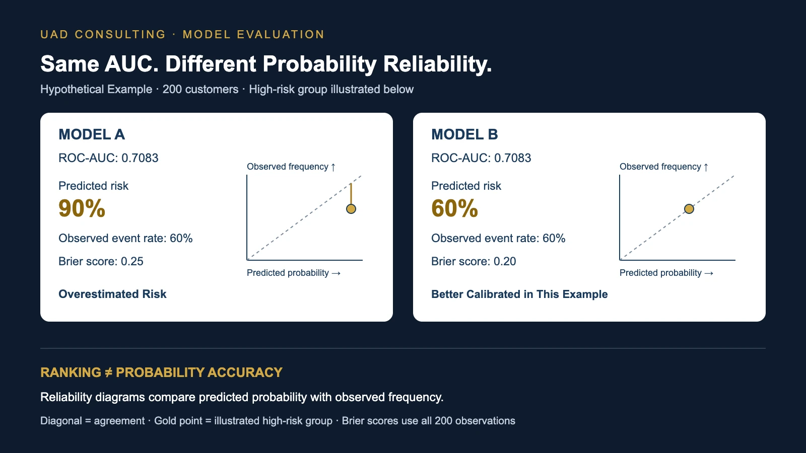
A Worked Example: Two Models With Identical AUC
Consider a hypothetical subscription company.
The business evaluates two machine learning models on the same 200 customers.
Exactly 80 customers cancel their subscriptions during the defined outcome period.
The remaining 120 do not.
For simplicity, divide the customers into two groups.
The lower-risk group contains 100 customers.
The higher-risk group also contains 100 customers.
Observed outcomes are:
| Group | Customers | Actual Churns | Actual Churn Rate |
|---|---|---|---|
| Lower risk | 100 | 20 | 20% |
| Higher risk | 100 | 60 | 60% |
| Total | 200 | 80 | 40% |
These observations are hypothetical.
They are constructed to demonstrate probability calibration.
Now suppose the two models produce different probability estimates.
Model A
Model A predicts:
Lower-risk group: 10%
Higher-risk group: 90%
Model B
Model B predicts:
Lower-risk group: 20%
Higher-risk group: 60%
Compare the predictions with the observed outcomes.
| Group | Actual Churn Rate | Model A Prediction | Model B Prediction |
|---|---|---|---|
| Lower risk | 20% | 10% | 20% |
| Higher risk | 60% | 90% | 60% |
Model A correctly assigns higher scores to the higher-risk group.
But its probability estimates are poorly calibrated.
It underestimates the lower-risk group's churn frequency.
It substantially overestimates the higher-risk group's churn frequency.
Model B assigns the same relative ranking.
However, its predicted probabilities match the observed frequencies in both groups.
This is the central distinction.
Both models separate the two groups in exactly the same order.
But the numerical meaning of their predictions differs.
Why Do Both Models Have the Same AUC?
AUC evaluates ranking.
In this example, both models assign the same score to every customer within a group.
Both models also assign a higher score to every customer in the higher-risk group than to every customer in the lower-risk group.
Therefore, they generate identical pairwise rankings.
Changing the lower-risk group's score from 0.10 to 0.20 does not change its position relative to the higher-risk group.
Changing the higher-risk group's score from 0.90 to 0.60 also preserves the ranking.
As a result, both models have:
ROC-AUC ≈ 0.7083
We can verify this directly.
There are:
80 positive observations
120 negative observations
Total positive-negative pairs:
80 × 120 = 9,600
The higher-risk group contains:
60 positive observations
40 negative observations
The lower-risk group contains:
20 positive observations
80 negative observations
Correctly ordered cross-group pairs:
60 × 80 = 4,800
Within-group pairs receive half credit because observations within each group have identical scores.
Lower-risk ties:
20 × 80 × 0.5 = 800
Higher-risk ties:
60 × 40 × 0.5 = 1,200
Total pairwise credit:
4,800 + 800 + 1,200 = 6,800
Therefore:
AUC = 6,800 / 9,600
AUC ≈ 0.7083
Both models produce this result.
Their ranking performance is identical.
Their probability calibration is not.
This demonstrates why AUC alone cannot determine whether predicted probabilities are suitable for financial or operational decision-making.
How Do We Measure Probability Accuracy?
One commonly used metric is the Brier score.
For binary outcomes, the Brier score measures the average squared difference between predicted probabilities and observed outcomes.
The formula is:
Brier Score = (1/N) × SUM((p_i - y_i)²)
Where:
N = Number of observations
p_i = Predicted probability for observation i
y_i = Actual binary outcome, either 0 or 1
A lower Brier score is better.
A score of zero represents perfect probabilistic predictions for the observed outcomes.
However, the Brier score is not a pure measure of calibration.
It also reflects discrimination, or resolution, and the underlying uncertainty of the outcome.
Therefore, a lower Brier score does not automatically prove that one model is better calibrated in every probability range.
Calibration curves and other diagnostics remain important.
For our example, the Brier score provides a useful numerical comparison because the two models are evaluated on the same observations.
Calculate the Brier Score for Model A
Model A predicts:
0.10 for every customer in the lower-risk group.
0.90 for every customer in the higher-risk group.
Start with the lower-risk group.
There are 20 customers who churn and 80 who do not.
For customers who churn:
Squared error = (0.10 - 1)²
= 0.81
For customers who do not churn:
Squared error = (0.10 - 0)²
= 0.01
Total squared error for the lower-risk group:
20 × 0.81 + 80 × 0.01
= 16.2 + 0.8
= 17
Now consider the higher-risk group.
There are 60 customers who churn and 40 who do not.
For customers who churn:
Squared error = (0.90 - 1)²
= 0.01
For customers who do not churn:
Squared error = (0.90 - 0)²
= 0.81
Total squared error:
60 × 0.01 + 40 × 0.81
= 0.6 + 32.4
= 33
Combine the groups:
Total squared error = 17 + 33
= 50
Divide by 200 observations:
Brier Score A = 50 / 200
Brier Score A = 0.25
Calculate the Brier Score for Model B
Model B predicts:
0.20 for the lower-risk group.
0.60 for the higher-risk group.
For the lower-risk group:
20 × (0.20 - 1)²
+
80 × (0.20 - 0)²
= 20 × 0.64 + 80 × 0.04
= 12.8 + 3.2
= 16
For the higher-risk group:
60 × (0.60 - 1)²
+
40 × (0.60 - 0)²
= 60 × 0.16 + 40 × 0.36
= 9.6 + 14.4
= 24
Total squared error:
16 + 24 = 40
Divide by 200:
Brier Score B = 40 / 200
Brier Score B = 0.20
The comparison is:
| Metric | Model A | Model B |
|---|---|---|
| ROC-AUC | 0.7083 | 0.7083 |
| Brier score | 0.25 | 0.20 |
| Lower-risk prediction | 10% | 20% |
| Lower-risk observed rate | 20% | 20% |
| Higher-risk prediction | 90% | 60% |
| Higher-risk observed rate | 60% | 60% |
Model B has the lower Brier score.
It also matches the observed event frequencies in the two constructed groups.
Model A overstates risk for one group and understates it for the other.
Yet the two models have identical AUC.
Compare Both Models With a Simple Baseline
A useful evaluation should also consider whether a model improves upon a reasonable baseline.
In our hypothetical dataset:
80 of 200 customers churn.
The overall churn rate is:
80 / 200 = 0.40
A simple baseline model could assign every customer a predicted churn probability of 40%.
Its Brier score is:
80 × (0.40 - 1)²
+
120 × (0.40 - 0)²
all divided by 200.
Calculate:
80 × 0.36 = 28.8
120 × 0.16 = 19.2
Total = 48
Brier Score = 48 / 200
= 0.24
Compare the results.
| Model | AUC | Brier Score |
|---|---|---|
| Model A | 0.7083 | 0.25 |
| Model B | 0.7083 | 0.20 |
| Constant 40% baseline | 0.50 | 0.24 |
Model A has better discrimination than the constant baseline.
Yet its Brier score is worse.
Model B improves on the baseline's Brier score.
This illustrates why a model evaluation should include multiple dimensions.
A model can add ranking information while producing probability estimates that are too extreme.
The comparison does not establish that Model B will remain superior in future data.
The example was deliberately constructed.
A real evaluation requires independent observations representing the intended deployment population.
Why Does Probability Calibration Matter for Business Decisions?
Suppose the subscription company uses predicted churn probabilities to decide whether to offer customers a retention intervention.
The intervention has a cost.
Management wants to apply it only when the expected avoided loss exceeds that cost.
For this illustration, assume:
Intervention cost per customer: $70
Avoidable loss if a customer churns: $100
Intervention effectiveness: 100% for customers who would otherwise churn
These are hypothetical assumptions.
Real retention interventions are rarely perfectly effective.
The example uses perfect effectiveness to isolate the relationship between probability calibration and decision-making.
The expected avoided loss for a customer is:
Predicted Churn Probability × $100
The intervention is financially attractive when:
Predicted Churn Probability × $100 > $70
Therefore:
Predicted Churn Probability > 0.70
The break-even probability is 70%.
This is an economic decision threshold.
It is not a universal machine learning classification threshold.
For the related policy-selection problem, see how classification thresholds affect business cost.
Model A and Model B Recommend Different Actions
Consider the higher-risk group.
Model A predicts a churn probability of 90%.
Its expected avoided loss is:
0.90 × $100 = $90
Subtract the intervention cost:
$90 - $70 = $20
Under Model A's predicted probability, the intervention appears to have an expected net benefit of $20 per customer.
Management would intervene.
Now consider Model B.
It predicts a churn probability of 60%.
Expected avoided loss:
0.60 × $100 = $60
Subtract the intervention cost:
$60 - $70 = -$10
Under Model B, the intervention has a negative expected net benefit.
Management would not intervene.
The models produce different decisions.
Yet their AUC scores are identical.
This is why probability calibration matters when decisions depend on expected financial outcomes.
What Happens Under the Observed Outcomes?
The higher-risk group contains 100 customers.
Exactly 60 actually churn in the hypothetical dataset.
Suppose management follows Model A and intervenes with all 100 customers.
Intervention cost:
100 × $70 = $7,000
Under the assumed perfect effectiveness, the intervention prevents the losses associated with all 60 customers who would otherwise churn.
Avoided loss:
60 × $100 = $6,000
Net financial result relative to no intervention:
$6,000 - $7,000
= -$1,000
Under these assumptions, intervening creates $1,000 more cost than doing nothing.
Model A predicted that intervention would be beneficial.
But its overestimated churn probabilities distorted the expected-cost calculation.
Model B's 60% prediction is consistent with the observed frequency in this constructed group.
It correctly indicates that the modeled intervention cost exceeds the expected avoided loss.
The important distinction is not that Model B is guaranteed to make better decisions in every setting.
It is that reliable probabilities are necessary when the decision rule depends directly on expected risk.
This example also assumes that the observed churn outcomes represent the counterfactual outcomes without intervention.
A real business must estimate intervention effectiveness separately.
AUC Cannot Tell You Whether an Intervention Works
Probability calibration addresses predictive reliability.
It does not establish causal intervention effectiveness.
Suppose a model accurately predicts that a customer has an 80% probability of churn.
That prediction does not establish that offering a discount will prevent the customer from leaving.
The customer may be highly likely to churn but unresponsive to the intervention.
Another customer may have a lower churn probability but be highly responsive to an offer.
These are different questions.
A churn model estimates:
P(Churn | Customer Characteristics)
A causal intervention model attempts to estimate how an action changes the outcome.
For example:
P(Churn Without Intervention)
versus
P(Churn With Intervention)
The difference between those potential outcomes represents the intervention's causal effect under the relevant assumptions.
A well-calibrated churn probability is not a substitute for estimating treatment effectiveness.
Randomized experiments or appropriately designed causal evaluations may be needed to estimate incremental intervention effects.
This distinction matters in marketing, healthcare, fraud prevention, and other decision systems.
Prediction tells us what may happen.
Causal analysis investigates what an intervention changes.
Decision analysis determines which action is preferable given the evidence, costs, benefits, and constraints.
How Do You Evaluate Probability Calibration?
A useful calibration evaluation should include several complementary methods.
1. Reliability Diagrams
A reliability diagram compares predicted probabilities with observed outcome frequencies.
For example, predictions can be grouped into probability intervals.
For each group, calculate:
Average predicted probability.
Observed event frequency.
Then plot:
Horizontal axis: Average predicted probability.
Vertical axis: Observed event frequency.
A perfectly calibrated model would lie along the diagonal line where:
Observed Frequency = Predicted Probability
If a point lies below the diagonal, the model is overestimating risk in that region.
If it lies above the diagonal, the model is underestimating risk.
However, calibration curves are estimates.
Their appearance depends on sample size, binning strategy, and the distribution of predictions.
A small sample can produce noisy results.
A curve that looks close to the diagonal does not prove perfect calibration.
2. Brier Score
The Brier score evaluates squared probability error.
It is useful for comparing probabilistic predictions on the same appropriately defined evaluation population.
However, it combines information about calibration, resolution, and outcome uncertainty.
A lower Brier score should not be interpreted as proof of better calibration in every subgroup.
3. Log Loss
Log loss is another proper scoring rule for probabilistic classification.
It penalizes predictions that assign very low probability to outcomes that actually occur.
Extremely confident incorrect predictions can produce large penalties.
Log loss can therefore be particularly sensitive to severe overconfidence.
The metric should be interpreted alongside calibration plots and relevant business outcomes.
4. Calibration Intercept and Slope
Calibration can also be assessed using a regression-based framework.
The calibration intercept helps assess systematic overprediction or underprediction.
The calibration slope helps assess whether predictions are too extreme or insufficiently differentiated.
An ideal intercept and slope depend on the exact parameterization, but commonly used logistic calibration models target an intercept of zero and a slope of one.
These measures can provide useful diagnostics.
However, they do not replace a careful examination of calibration across the prediction range.
5. Subgroup Calibration
A model may appear well calibrated overall while performing poorly for important subgroups.
For example, calibration may differ by:
Customer segment.
Product category.
Geographic region.
Acquisition channel.
Time period.
Clinical population.
Operational setting.
The relevant subgroups should be defined according to the intended decision and applicable fairness, privacy, and governance requirements.
Small subgroup samples require particular caution.
Reproduce the Example in Python
The following Python code reproduces the hypothetical 200-customer example.
It uses synthetic observations.
No real customer or healthcare data are required.
import numpy as np

from sklearn.metrics import (
    roc_auc_score,
    brier_score_loss
)

# Hypothetical observed outcomes

# Lower-risk group:
# 20 churns, 80 non-churns

low_risk_outcomes = np.array(
    [1] * 20 + [0] * 80
)

# Higher-risk group:
# 60 churns, 40 non-churns

high_risk_outcomes = np.array(
    [1] * 60 + [0] * 40
)

y_true = np.concatenate([
    low_risk_outcomes,
    high_risk_outcomes
])

# Model A probabilities

model_a = np.concatenate([
    np.full(100, 0.10),
    np.full(100, 0.90)
])

# Model B probabilities

model_b = np.concatenate([
    np.full(100, 0.20),
    np.full(100, 0.60)
])

# Constant baseline probability

baseline = np.full(
    len(y_true),
    y_true.mean()
)

for name, probabilities in [
    ("Model A", model_a),
    ("Model B", model_b),
    ("Baseline", baseline)
]:

    auc = roc_auc_score(
        y_true,
        probabilities
    )

    brier = brier_score_loss(
        y_true,
        probabilities
    )

    print(
        name,
        "AUC:",
        round(auc, 4),
        "Brier:",
        round(brier, 4)
    )
Expected output:
Model A: AUC = 0.7083 Brier = 0.2500
Model B: AUC = 0.7083 Brier = 0.2000
Baseline: AUC = 0.5000 Brier = 0.2400
These results demonstrate that two models can have identical ranking performance while producing different probability errors.
The example is deliberately simple.
It should not be interpreted as a production model validation.
How Can Poorly Calibrated Probabilities Be Improved?
Several methods can be used to calibrate model probabilities.
Two established approaches are sigmoid calibration and isotonic regression.
Sigmoid Calibration
Sigmoid calibration fits a parametric mapping between model scores and observed outcomes.
It is often associated with Platt scaling.
The method can be useful when the relationship between raw scores and observed probabilities is reasonably represented by a sigmoid-shaped transformation.
Its parametric structure can be helpful when calibration data are limited.
However, the assumed functional form may not fit every model.
Isotonic Regression
Isotonic regression fits a nondecreasing transformation of model scores.
It is more flexible than a fixed sigmoid mapping.
That flexibility can help when the calibration relationship has an irregular shape.
However, isotonic regression can overfit when calibration data are limited.
It can also create tied calibrated probabilities.
The appropriate method depends on the amount of calibration data, model behavior, and validation results.
Neither approach should be assumed superior without evaluation.
Preserve Independent Evaluation
Calibration methods learn from observed outcomes.
Therefore, the data used to fit the calibration transformation should be separated appropriately from the data used for final evaluation.
A calibration model fitted and evaluated on the same observations can appear artificially successful.
Cross-validation and properly separated calibration datasets can reduce this problem.
The official scikit-learn documentation provides tools such as CalibratedClassifierCV and calibration_curve.
The exact implementation should follow the relevant software version and validation design.
Does Calibration Change AUC?
Not necessarily.
A strictly increasing transformation preserves the ranking of model scores.
Therefore, a strictly increasing calibration mapping leaves ROC-AUC unchanged.
This is why probability calibration can improve numerical probability reliability without improving ranking discrimination.
However, not every calibration transformation is strictly increasing.
For example, isotonic regression can assign identical calibrated probabilities to observations that previously had different scores.
These new ties can affect AUC.
Therefore, it would be incorrect to claim that every calibration procedure always preserves ROC-AUC exactly.
The important distinction is that calibration primarily addresses probability reliability, while discrimination evaluates ranking.
A model evaluation should measure both after any transformation.
What Happens When the Outcome Rate Changes?
A model calibrated on historical data may become poorly calibrated when the deployment population changes.
Suppose a churn model was calibrated when the overall churn rate was 20%.
Six months later, the company changes its subscription policy.
The customer population also changes.
The observed churn rate rises to 35%.
The model's previous probability mapping may no longer describe the current population accurately.
This does not automatically mean the ranking model has become useless.
A model can retain useful discrimination while its calibration deteriorates.
The appropriate response depends on the cause.
Possible responses include:
Investigating data quality.
Checking whether outcome definitions changed.
Reassessing the deployment population.
Updating the calibration mapping.
Reevaluating the classification threshold.
Retraining the underlying model when justified.
These are different interventions.
Retraining should not be the automatic response to every calibration problem.
For a broader discussion, see UAD Consulting's article on when to retrain a machine learning model.
Why Calibration Must Be Evaluated at the Right Time
Prediction timing matters.
Suppose a business predicts whether a customer will cancel during the next 30 days.
The model is evaluated using historical data.
However, some predictors were updated after the prediction date.
The resulting evaluation may use information that would not have been available when the prediction was originally required.
This creates a data-leakage problem.
Calibration results obtained under leaked or unrealistic evaluation conditions may not represent future performance.
A defensible evaluation should specify:
The prediction timestamp.
The outcome window.
The population being scored.
The features available at prediction time.
The training period.
The calibration period.
The independent evaluation period.
The handling of delayed outcomes.
For related methodology, see UAD Consulting's article on data leakage in machine learning.
A Practical Calibration Monitoring Dashboard
A production model should not be monitored using AUC alone.
A useful monitoring framework can include:
| Dimension | Example Metric | Management Question |
|---|---|---|
| Discrimination | ROC-AUC | Does the model rank outcomes effectively? |
| Probability quality | Brier score | How accurate are the probability forecasts overall? |
| Calibration | Reliability diagram | Do predicted risks match observed frequencies? |
| Calibration summary | Intercept and slope | Is risk systematically misestimated? |
| Population | Outcome prevalence | Has the underlying event rate changed? |
| Operational use | Action rate | How many cases trigger intervention? |
| Economics | Expected decision cost | Are actions economically justified? |
| Data quality | Missing features | Can predictions be trusted operationally? |
These measures should be interpreted together.
A stable AUC does not guarantee stable calibration.
A lower Brier score does not guarantee better calibration at every decision threshold.
A calibrated probability does not establish intervention effectiveness.
And a favorable expected-cost model does not guarantee realized savings.
Each metric answers a different question.
A Practical Framework for Using Model Probabilities
Before using predicted probabilities in an operational decision, answer seven questions.
1. What Outcome Is Being Predicted?
Define the target and prediction horizon precisely.
For example:
Customer cancellation within 30 days.
Payment default within 12 months.
Equipment failure within seven days.
The meaning of a predicted probability depends on the outcome definition.
2. Is the Evaluation Population Representative?
Determine whether the validation data resemble the population where the model will be used.
Check for selection bias, population changes, and important subgroup differences.
3. Does the Model Discriminate?
Evaluate ranking performance using metrics appropriate to the prediction task.
ROC-AUC may be useful, but it should not be the only measure.
4. Are the Probabilities Calibrated?
Compare predicted probabilities with observed frequencies.
Use calibration curves and appropriate quantitative diagnostics.
Examine uncertainty when sample sizes are limited.
5. What Decision Uses the Probability?
Identify the action triggered by the model.
For example:
Contact a customer.
Review a transaction.
Inspect a machine.
Prioritize an operational case.
The decision determines which probability ranges matter most.
6. What Are the Costs and Benefits?
Estimate relevant action costs and consequences.
Do not assume that the predicted event probability equals the probability that an intervention will succeed.
7. How Will the Model Be Monitored?
Define how calibration, discrimination, data quality, and business outcomes will be evaluated after deployment.
A model that is reliable today may require updating when the environment changes.
Frequently Asked Questions
Can a model have good AUC but poor calibration?
Yes.
AUC measures ranking discrimination.
Calibration measures agreement between predicted probabilities and observed outcome frequencies.
A model can rank observations correctly while systematically overestimating or underestimating risk.
Does probability calibration improve model accuracy?
It can improve probability reliability, but it does not necessarily improve classification accuracy or ROC-AUC.
The effect depends on the calibration method, model, and evaluation data.
What is a good Brier score?
Lower is better, but there is no universally meaningful cutoff across all prediction problems.
Interpret the score relative to the outcome prevalence, relevant baselines, alternative models, and the decision context.
Is a lower Brier score proof of better calibration?
No.
The Brier score reflects multiple aspects of probabilistic prediction quality, including calibration and resolution.
Use calibration curves and additional diagnostics.
What is a reliability diagram?
A reliability diagram compares predicted probabilities with observed outcome frequencies across groups of predictions.
It helps identify overconfidence and underconfidence.
Should every machine learning model be calibrated?
Not necessarily.
Calibration is especially important when predicted probabilities are interpreted as risks or used directly in expected-value calculations.
For applications that use only ranking, calibration may be less central, although it can still be useful.
Can a calibrated model tell us which intervention will work?
No.
Calibration evaluates predicted outcome probabilities.
Estimating intervention effectiveness requires additional causal evidence.
The Most Important Question Is What the Probability Means
Return to our hypothetical subscription company.
Two models evaluate the same 200 customers.
Both have an AUC of approximately 0.7083.
Both rank the higher-risk group above the lower-risk group.
But Model A predicts a 90% churn probability for a group whose observed churn frequency is 60%.
Model B predicts 60%.
The models have identical ranking performance.
Yet their probability estimates support different expected-cost decisions.
Under the illustrative intervention assumptions, acting on Model A's overestimated risk creates a modeled financial disadvantage.
Model B's better-calibrated probabilities avoid that particular mistake.
The lesson extends beyond customer churn.
Machine learning models are often used to estimate risks, prioritize resources, and support decisions under uncertainty.
A model can provide useful rankings without providing reliable probabilities.
When decisions depend on expected outcomes, that distinction matters.
The objective is not simply to achieve a high AUC.
It is to produce predictions that are reliable enough for their intended use and connect those predictions to defensible decisions.
That requires evaluating discrimination, calibration, operational constraints, intervention effectiveness, and business consequences.
A trustworthy predictive system is not defined by one impressive metric.
It is defined by whether its outputs can be interpreted and used appropriately.
References and Further Reading
- Scikit-learn Developers. Probability Calibration. Official scikit-learn User Guide.
- Scikit-learn Developers. sklearn.calibration API Reference.
- Van Calster B, McLernon DJ, van Smeden M, Wynants L, Steyerberg EW. (2019). Calibration: The Achilles Heel of Predictive Analytics. BMC Medicine, 17, 230.
- Scikit-learn Developers. Brier Score Loss. Official API documentation.
All numerical examples are hypothetical.
They are provided for educational purposes and do not represent actual client data, observed consulting results, or guaranteed improvements from machine learning.
Make Predictive Models More Decision-Ready
A machine learning model is valuable when its outputs can support reliable and defensible decisions.
UAD Consulting helps organizations connect statistical modeling, predictive analytics, model evaluation, and decision analysis to practical business problems.
Whether the challenge involves classification, probability calibration, operational risk, or translating predictions into economic decisions, the objective is to understand what the model can support and where its limitations matter.
Explore our Data Science & Machine Learning services to discuss your predictive analytics and decision-modeling needs.
Explore ServicesGet in Touch