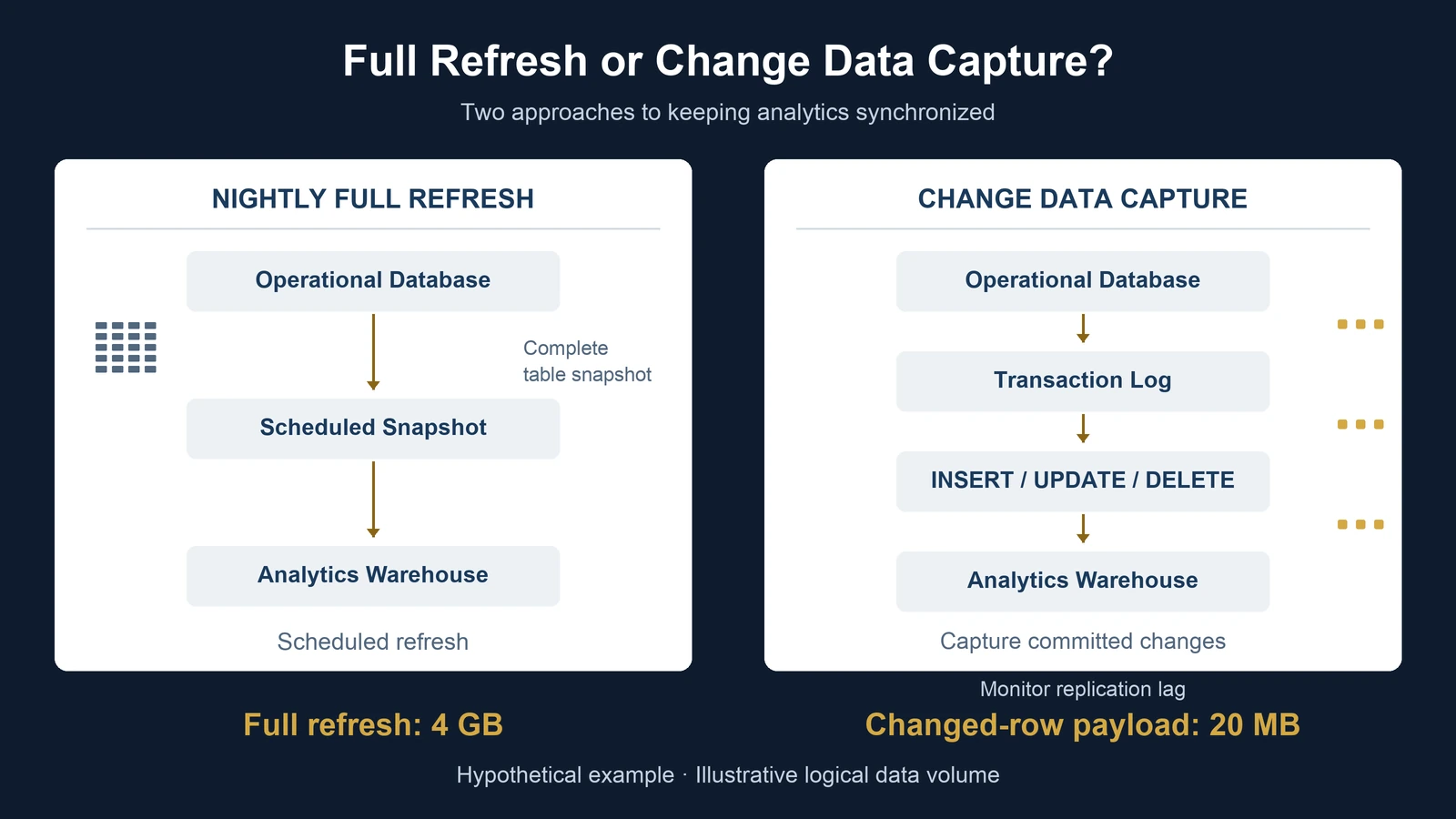
A company operates an online store.
Orders are recorded in its operational database.
A separate analytics database supports management dashboards, revenue reporting, customer analysis, and inventory planning.
Every night, the company copies its order data into the analytics environment.
The process works.
But as the business grows, the nightly refresh takes longer. Managers increasingly ask for updated information during the day, and the engineering team begins considering Change Data Capture, commonly called CDC.
Should the company replace its nightly process with a continuous data pipeline?
Not necessarily.
The decision depends on how frequently the business needs updated information, how much data changes, whether updates and deletions must be preserved, and how much operational complexity the organization can support.
A nightly refresh may be entirely sufficient for financial reporting.
An hourly incremental load may support inventory planning.
A continuously running CDC pipeline may be appropriate when operational decisions depend on recent database changes.
The important question is not which architecture sounds more advanced.
It is which architecture provides the required data freshness, correctness, reliability, and recoverability at a reasonable total cost.
The Short Answer: Choose the Simplest Pipeline That Meets the Decision Requirement
There are three common approaches to keeping analytical data synchronized with operational systems.
Full refresh replaces or reconstructs the analytical dataset using a complete source snapshot.
Incremental loading extracts records that have changed since a previous extraction, often using a source-maintained modification timestamp or another change-tracking mechanism.
Change Data Capture identifies database changes, often through transaction logs, and makes those changes available to downstream systems.
These approaches are not mutually exclusive.
A business might initially load an entire table and then use CDC to maintain it.
Another business might run hourly incremental loads and periodically perform full reconciliation.
A third might use nightly full refreshes for financial reporting and CDC for operational order monitoring.
The right architecture is often a combination rather than a universal standard.
What Is a Full Data Refresh?
A full refresh reads the relevant source dataset and reconstructs its analytical representation.
Consider an operational database containing eight million order records.
A nightly pipeline might:
- Read all eight million records.
- Transfer them into a staging environment.
- Validate row counts, required fields, and business rules.
- Replace the previous analytical snapshot.
- Make the refreshed data available to dashboards.
The process is conceptually straightforward.
A properly implemented full refresh can reflect inserts, updates, and deletions because it reconstructs the current source state.
However, that requires the source extract to be complete and consistent.
Deleting the existing analytical table before confirming that a replacement extract succeeded can leave dashboards empty or incomplete.
A safer pattern is to load a separate staging table, validate it, and then perform a controlled replacement or swap.
The precise implementation depends on the database and warehouse.
When Full Refresh Works Well
Full refresh can be appropriate when:
- The dataset is relatively small.
- Daily reporting is sufficient.
- The extraction finishes within its required window.
- Source systems can tolerate the extraction workload.
- Operational simplicity is important.
- Current-state reporting matters more than a complete history of changes.
For example, a small business producing a weekly executive dashboard may not need a continuously running replication system.
A reliable nightly extract could provide everything required.
When Full Refresh Becomes Difficult
As data grows, repeatedly reading unchanged records can become expensive or operationally disruptive.
A full refresh may consume:
- Source database resources.
- Network bandwidth.
- Warehouse ingestion capacity.
- Processing time.
- Storage and temporary staging resources.
It can also create a long interval between source changes and analytical availability.
But these problems are not inevitable.
Columnar storage, partitioning, efficient exports, source replicas, and other architectural choices can make full refreshes practical even for substantial datasets.
The decision requires measurement rather than a fixed row-count threshold.
What Is Incremental Loading?
Incremental loading attempts to extract only records that are new or have changed since the previous successful extraction.
A common implementation uses an updated_at column.
Suppose the orders table contains:
- order_id
- customer_id
- amount_usd
- status
- updated_at
- deleted_at
An incremental process may query records modified during a defined time window.
For example:
SELECT
    order_id,
    customer_id,
    amount_usd,
    status,
    updated_at,
    deleted_at
FROM orders
WHERE updated_at >= :lower_bound
  AND updated_at < :upper_bound
ORDER BY updated_at, order_id;
This example uses PostgreSQL-compatible SQL syntax and illustrative parameters.
The lower and upper bounds must be determined by the pipeline.
A robust implementation should establish a consistent source-side extraction boundary, replay a suitable overlap when necessary, and advance its durable checkpoint only after the destination update succeeds.
The query alone does not guarantee complete change capture.
The Advantages
Incremental loading can substantially reduce the amount of source data read and transferred.
It can also support more frequent refreshes without repeatedly copying the entire table.
For a business that needs hourly reporting, this may provide a useful balance between freshness and complexity.
The Hidden Problem: Deleted Records
Suppose an order is physically deleted from the source database.
A timestamp-based query against the current source table cannot return a row that no longer exists.
The analytical database may therefore retain a record that has been removed from the source.
Soft deletion can help when the source maintains a deletion indicator and updates its modification timestamp.
However, not every system supports that pattern.
Other options include source-provided deletion feeds, periodic reconciliation, or log-based CDC.
A timestamp-based incremental process must not be assumed to capture every type of database change.
Another Problem: Missed Updates
Modification timestamps can be unreliable if:
- Some application updates do not maintain the field.
- Different processes use inconsistent timestamps.
- Records are committed after an extraction boundary was established.
- Multiple updates share the same timestamp.
- Source clocks or timestamp precision create ambiguity.
- A failed extraction advances its checkpoint prematurely.
An overlap window and idempotent destination updates can reduce some risks.
They cannot recover every possible missing change.
If the source does not provide a trustworthy modification mechanism, timestamp-based extraction may be inappropriate.
What Is Change Data Capture?
Change Data Capture identifies changes made to source data and makes those changes available for downstream processing.
A common form is log-based CDC.
Many transactional databases maintain logs recording changes required for durability, recovery, or replication.
Depending on the database engine and connector, a CDC system can read committed changes from those logs.
Typical operations include:
- INSERT
- UPDATE
- DELETE
A simplified architecture is:
Operational Database
↓
Database Transaction Log
↓
CDC Connector
↓
Change Events
↓
Destination Apply Process
↓
Analytics Database or Warehouse
A CDC pipeline often begins with an initial snapshot of existing records.
It then continues processing changes made after the snapshot's established log position.
The snapshot and streaming phases must be coordinated so that changes occurring during initialization are not silently lost.
This is a key reason to use established CDC mechanisms rather than treating continuous replication as a collection of ordinary SQL queries.
CDC Does Not Automatically Mean Real Time
The term CDC is sometimes associated with real-time analytics.
That description can be misleading.
A CDC pipeline may experience delays because of:
- Source database workload.
- Transaction volume.
- Connector performance.
- Network interruptions.
- Destination processing capacity.
- Large transactions.
- Replication backlogs.
- Infrastructure failures.
AWS Database Migration Service explicitly documents that its CDC replication is not guaranteed to operate in real time.
Replication latency depends on the surrounding system.
Therefore, a business requiring updates within fifteen minutes should measure whether the complete pipeline meets that requirement.
It should not assume that installing a CDC connector guarantees fifteen-minute freshness.
A Worked Example: Eight Million Rows, but Only 0.5% Change Daily
Consider a hypothetical company with the following operational database characteristics.
| Assumption | Value |
|---|---|
| Current table size | 8,000,000 rows |
| Average logical row payload | 500 bytes |
| Daily changed rows | 40,000 |
| Daily change rate | 0.5% |
| Full refresh frequency | Once daily |
These are illustrative assumptions, not measured client data.
For simplicity, assume each changed row generates one relevant change event and use the same 500-byte logical row payload in both comparisons.
Actual CDC event payloads can differ substantially from full-row extracts.
Step 1: Calculate Full Refresh Volume
A complete refresh reads:
8,000,000 rows.
At an average logical payload of 500 bytes:
8,000,000 × 500
= 4,000,000,000 bytes.
Using decimal units:
4 GB.
The full refresh therefore transfers approximately 4 GB of logical row payload per run under the stated assumptions.
Step 2: Calculate Changed-Row Payload
Only 40,000 rows change during the day.
40,000 × 500
= 20,000,000 bytes.
Using decimal units:
20 MB.
Step 3: Compare the Volumes
Full refresh:
4,000 MB.
Changed-row payload:
20 MB.
Ratio:
4,000 / 20
= 200.
The illustrative full-refresh payload is 200 times the changed-row payload.
Equivalently, the changed-row payload represents 0.5% of the full dataset.
Step 4: Interpret the Result Correctly
This does not establish that CDC is 200 times cheaper.
The calculation compares logical data payload under simplified assumptions.
It does not estimate actual cloud billing or end-to-end infrastructure cost.
Real systems may incur additional costs from:
- CDC event envelopes.
- Before-and-after images.
- Transaction metadata.
- Log retention.
- Connector infrastructure.
- Message brokers.
- Destination writes.
- Transformation processing.
- Monitoring and recovery.
- Initial snapshots and periodic reconciliation.
Compression and columnar exports can also reduce the physical size of full-refresh transfers.
A business should therefore distinguish data volume from total operating cost.
The calculation demonstrates why incremental architectures may become attractive when a small fraction of a large dataset changes.
It does not prove that CDC is economically preferable.
The More Important Question: What Happens to Updates and Deletes?
Reducing transfer volume is only one part of the problem.
An analytical system must also represent the correct source state.
Consider a simplified order table.
At the beginning of the day:
| Order ID | Amount |
|---|---|
| 501 | $120 |
| 502 | $80 |
Initial total:
$120 + $80 = $200.
Three changes then occur.
| Time | Operation | Order | New State |
|---|---|---|---|
| 9:10 AM | UPDATE | 501 | $90 |
| 9:12 AM | DELETE | 502 | Removed |
| 9:15 AM | INSERT | 503 | $50 |
The correct final state is:
| Order ID | Amount |
|---|---|
| 501 | $90 |
| 503 | $50 |
Final total:
$90 + $50 = $140.
Why Simply Appending Changes Fails
Suppose an analyst treats the new CDC records as additional orders.
The analytical dataset could incorrectly contain:
$120 + $80 + $90 + $50
= $340.
The update has been counted as a new order.
The deleted order remains in the analytical total.
The pipeline may have received every event and still produced an incorrect dashboard.
This illustrates a fundamental distinction.
A stream of database changes is not automatically a correct current-state table.
The destination must interpret operations properly.
An UPDATE should modify the corresponding destination record.
A DELETE should remove or appropriately mark the corresponding record.
An INSERT should create a new record.
If the destination is intended to preserve historical changes, the events may instead be stored in an append-only history table.
But that history table should not be queried as though every event represents a separate current order.
The intended analytical data model determines the correct processing behavior.
CDC Requires Reliable Keys and Event Ordering
A destination must identify which source record each change affects.
Stable primary keys are therefore important.
For PostgreSQL logical replication, UPDATE and DELETE operations require an appropriate replica identity.
A primary key commonly provides that identity.
Without a suitable identity configuration, the system may not be able to replicate these operations correctly.
Event ordering also matters.
Suppose an order changes from:
$120 to $90.
Then from:
$90 to $70.
If the destination applies the events in the wrong order, it could incorrectly finish at $90.
A production pipeline must understand the ordering guarantees of its connector, transport, and destination.
Those guarantees may differ across database systems and infrastructure components.
Duplicate Events Are Possible
CDC pipelines can experience interruptions.
After recovery, a connector may replay events that were previously processed.
Debezium's PostgreSQL documentation explicitly discusses duplicate events during failure recovery.
A downstream consumer should therefore be designed to handle replay safely.
This is often called idempotent processing.
In practical terms, applying the same logical change again should not incorrectly duplicate its business effect.
The implementation may use:
- Stable record identifiers.
- Source log positions.
- Event sequence information.
- Version-aware updates.
- Deduplication logic.
- Transactional destination writes.
The correct method depends on the source and destination.
Exactly-once business outcomes should not be assumed merely because a connector advertises delivery guarantees.
Full Refresh, Incremental Loading, and CDC Compared
The following table summarizes the practical differences.
| Dimension | Full Refresh | Incremental Loading | Log-Based CDC |
|---|---|---|---|
| Typical extraction | Complete snapshot | Selected changed records | Database change stream |
| Refresh frequency | Scheduled | Scheduled or frequent | Continuously processed |
| Hard deletes | Reflected by complete replacement | Usually need additional handling | Can be captured if supported and configured |
| Source requirements | Consistent extraction | Reliable change marker | Log access and replication configuration |
| Initial implementation | Often simplest | Moderate | Often more complex |
| Recovery | Rebuild snapshot | Replay or backfill | Resume log position or resnapshot |
| Main risk | Heavy repeated extraction | Missed changes | Replication gaps, lag, operational complexity |
| Best fit | Tolerant freshness requirements | Moderate freshness requirements | Frequent updates with strong change-capture needs |
These are general architectural tendencies.
Specific database engines, managed services, and pipeline designs may behave differently.
For example, an incremental pipeline using a reliable source-provided change feed can capture deletes without using database transaction logs.
Likewise, a full refresh can be implemented with sophisticated partitioning and staging.
The labels alone do not determine reliability.
When Is a Nightly Refresh Actually Enough?
Consider a company whose finance team reviews yesterday's completed transactions every morning.
The dashboard is used at 9:00 AM.
The source extract starts at 2:00 AM and completes successfully by 3:00 AM.
Suppose the business has explicitly determined that data through the prior reporting cutoff is sufficient.
In this situation, a nightly refresh may satisfy the decision requirement.
Moving to CDC could add:
- Connector administration.
- Continuous monitoring.
- Additional failure modes.
- Log retention requirements.
- More complicated recovery procedures.
If the extra freshness does not change a meaningful business decision, the investment may have little value.
The relevant question is:
"What would we do differently if this information were available sooner?"
If there is no clear answer, faster ingestion may not be a priority.
When Does CDC Become More Attractive?
Now consider a distributor monitoring orders, inventory allocations, and cancellations.
Operational managers need to react to changes throughout the day.
A dashboard that updates only once every night may be too stale for the decisions being made.
CDC may be worth evaluating when:
- Source changes are frequent.
- A small fraction of a large dataset changes at a time.
- Updates and hard deletes must be captured.
- The source supports reliable log-based change capture.
- The business has a meaningful freshness requirement.
- The organization can monitor and recover the pipeline.
- A simpler incremental approach cannot reliably meet the requirements.
Even then, CDC is not automatically the only solution.
Some businesses can meet their needs through hourly incremental extraction.
Others may use application events or a managed change feed.
The objective should be reliable decision support rather than architectural sophistication.
Define Freshness as a Measurable Service Requirement
A useful freshness requirement should specify more than "near real time."
For example:
"During business hours, 95% of committed order changes should become visible in the operational dashboard within fifteen minutes."
This statement identifies:
- The source event being measured.
- The destination where the change must appear.
- The latency threshold.
- The measurement percentile.
- The relevant operating period.
The team can then monitor end-to-end latency.
A simplified definition is:
Data availability latency = Destination visibility time - Source commit time.
The measurement should use comparable timestamps and account for clock synchronization.
Connector lag alone is insufficient if downstream transformations and dashboard refreshes introduce additional delays.
For example, a CDC connector may capture changes within seconds while the dashboard refreshes only once per hour.
The business still does not have a continuously updated dashboard.
Freshness must be evaluated across the complete system.
Reliability Matters More Than Refresh Frequency Alone
A pipeline that updates every minute but silently misses deletions may be less trustworthy than a validated daily refresh.
A useful monitoring framework includes:
| Control | Question |
|---|---|
| Freshness | How old is the latest available change? |
| Completeness | Were expected changes captured? |
| Uniqueness | Were records duplicated during replay? |
| Delete handling | Were removals reflected correctly? |
| Schema validation | Did source field definitions change? |
| Reconciliation | Does destination state agree with the source? |
| Recovery | Can the pipeline resume after interruption? |
| Observability | Can operators identify and explain failures? |
These controls are relevant across all three architectures.
For a broader discussion, see UAD Consulting's article on data quality checks for analytics pipelines.
Reconciliation Is Still Necessary With CDC
CDC does not eliminate the need to compare source and destination data.
A connector can remain active while a downstream transformation fails.
A schema change may cause a field to be interpreted incorrectly.
An event consumer may process updates but mishandle deletes.
A periodic reconciliation process can compare:
- Row counts.
- Primary-key coverage.
- Important financial totals.
- Record versions.
- Deleted-record status.
- Selected source and destination values.
For large datasets, reconciliation may use partitions, hashes, aggregates, or targeted samples.
The correct approach depends on the accuracy requirement and system design.
A successful CDC connector status is not proof that every business metric is correct.
CDC Also Changes Recovery Planning
A nightly full refresh has a relatively intuitive recovery mechanism.
If a refresh fails, the team may rerun the extraction and reconstruct the destination.
Incremental and CDC pipelines require more careful checkpoint management.
For CDC, the source must retain the necessary log history while the consumer is disconnected.
If the connector's required log position is no longer available, the system may need to establish a new snapshot or use another recovery mechanism.
Recovery planning should address:
- Maximum acceptable downtime.
- Available log retention.
- Checkpoint durability.
- Replay behavior.
- Duplicate-event handling.
- Initial snapshot consistency.
- Destination reconstruction.
- Schema compatibility.
A business should test these procedures before treating the pipeline as operationally critical.
How Should a Business Compare Total Cost?
Data transfer volume is only one cost component.
A practical comparison should include the full operating model.
Full Refresh Costs
Potential components include:
- Source extraction.
- Data transfer.
- Staging storage.
- Warehouse loading.
- Validation.
- Scheduled orchestration.
- Recovery after failures.
Incremental Loading Costs
Potential components include:
- Change-marker maintenance.
- Incremental extraction.
- Destination upserts.
- Delete detection.
- Checkpoint management.
- Periodic backfills.
- Reconciliation.
CDC Costs
Potential components include:
- Initial snapshot.
- Source replication configuration.
- Connector infrastructure.
- Transaction-log retention.
- Event transport.
- Destination event application.
- Monitoring.
- Recovery testing.
- Operational support.
The cheapest architecture is not necessarily the one with the fewest transferred bytes.
Nor is the architecture with the lowest infrastructure bill necessarily the best business choice.
The analysis should also consider the consequences of stale or incorrect data.
If a delayed inventory signal causes expensive operational errors, improved freshness may have economic value.
But that value must be estimated using explicit assumptions and evidence.
Does Faster Data Actually Improve Business Outcomes?
Suppose a company introduces CDC and subsequently observes fewer inventory shortages.
It would be tempting to conclude that CDC caused the improvement.
That conclusion may be premature.
During the same period, the company might have:
- Changed suppliers.
- Increased safety stock.
- Updated forecasting models.
- Modified replenishment rules.
- Experienced different demand conditions.
- Improved warehouse operations.
The observed association does not isolate the effect of faster data availability.
A decision model can estimate how different data delays might affect inventory decisions under specified assumptions.
A controlled rollout or carefully designed comparison may provide stronger evidence of operational impact.
The distinction matters.
Data engineering improves the availability and structure of information.
Decision modeling estimates the consequences of alternative actions.
Causal evaluation asks whether an intervention actually changed outcomes.
These are related but different analytical questions.
Fresh data does not resolve conflicting planning totals; forecast reconciliation across regions addresses that separate consistency problem.
A Practical Five-Step Decision Framework
Organizations can evaluate their data refresh architecture through five steps.
Step 1: Identify the Business Decision
Which recurring decision depends on the data?
Examples include:
- Daily financial reporting.
- Hourly inventory planning.
- Order exception monitoring.
- Customer support prioritization.
- Operational capacity allocation.
The decision should determine the required freshness.
Step 2: Measure the Current Pipeline
Record:
- Source row counts.
- Data volume.
- Daily change rate.
- Extraction duration.
- Source workload.
- Failure frequency.
- Actual end-to-end freshness.
Do not select a new architecture based solely on assumed performance.
Step 3: Examine Source Change Semantics
Determine whether the source supports:
- Reliable modification timestamps.
- Stable primary keys.
- Soft deletion.
- Hard deletion tracking.
- Transaction-log access.
- Consistent snapshots.
- Sufficient log retention.
These characteristics determine which extraction methods are trustworthy.
Step 4: Compare Architecture Options
Evaluate full refresh, incremental loading, and CDC against the same requirements.
Consider:
- Correctness.
- Freshness.
- Recovery.
- Complexity.
- Security.
- Operating cost.
- Maintenance responsibility.
Use a small pilot when the preferred option is uncertain.
Step 5: Validate Business Value
Determine whether the proposed improvement changes decisions enough to justify its cost.
A faster pipeline may be valuable.
A simpler pipeline may be sufficient.
The correct recommendation depends on the organization's requirements, not the popularity of a technology.
For a related architectural discussion, see When Does a Business Actually Need a Data Warehouse?.
The Bottom Line: Freshness Is a Requirement, Not an Architecture
A full refresh, incremental load, and CDC pipeline can all support reliable analytics when implemented appropriately.
Full refresh offers a straightforward way to reconstruct current source state.
Incremental loading can reduce repeated extraction when trustworthy change markers are available.
CDC can capture committed database changes and support more frequent synchronization, but it introduces additional operational responsibilities.
Our hypothetical eight-million-row example demonstrates why avoiding repeated full-table transfers may be attractive.
Under the stated assumptions, the changed-row payload is only 0.5% of the full dataset.
But lower payload does not automatically mean lower total cost, better reliability, or better business outcomes.
The strongest architecture begins with a measurable decision requirement.
How fresh must the data be?
Which changes must be captured?
How will correctness be verified?
How will failures be recovered?
And what business decision becomes better because the information arrives sooner?
The objective is not to move data as quickly as possible.
It is to make the right information available, accurately and reliably, when a decision requires it.
References and Methodological Notes
Amazon Web Services.
AWS Database Migration Service: Creating Tasks for Ongoing Replication.
https://docs.aws.amazon.com/dms/latest/userguide/CHAP_Task.CDC.html
Official documentation describing full-load and CDC replication, source log requirements, and latency limitations.
Debezium.
Debezium Connector for PostgreSQL.
https://debezium.io/documentation/reference/stable/connectors/postgresql.html
Technical documentation covering snapshots, streaming changes, source log positions, duplicate events, and recovery behavior.
PostgreSQL Global Development Group.
PostgreSQL Documentation: Logical Replication — Publication.
https://www.postgresql.org/docs/current/logical-replication-publication.html
Official documentation describing publication operations and replica identity requirements for UPDATE and DELETE replication.
Amazon Web Services.
Best Practices for AWS Database Migration Service.
https://docs.aws.amazon.com/dms/latest/userguide/CHAP_BestPractices.html
Guidance on CDC latency, infrastructure requirements, and ongoing replication considerations.
Methodological Note
All business examples and numerical calculations in this article are hypothetical.
They do not represent actual UAD Consulting client data or measured production outcomes.
The 4 GB versus 20 MB example compares simplified logical row payloads.
It excludes physical storage formats, compression, CDC event overhead, infrastructure costs, and other implementation-specific factors.
The SQL example is an illustrative extraction pattern, not a complete production-ready ingestion system.
Database replication behavior varies by engine, connector, version, configuration, and destination.
Build an Analytics Pipeline You Can Trust
Reliable reporting starts with a data architecture that fits the business.
UAD Consulting helps organizations examine data sources, SQL workflows, integration requirements, and data-quality controls to support dependable analytics and decision-making.
Explore our Data Engineering & Database Analytics services or get in touch to discuss your reporting and data integration challenges.
Explore ServicesGet in Touch