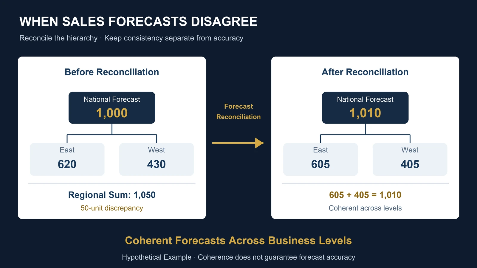
A company prepares its sales forecast for the next quarter.
The finance department expects 1,000 units to be sold.
The East regional manager forecasts 620 units.
The West regional manager forecasts 430 units.
There is a problem.
The two regional forecasts add up to 1,050 units.
But the company-wide forecast is only 1,000.
Both forecasts cannot be used simultaneously as one internally consistent plan.
If management adopts the national forecast, regional allocations may not match.
If it adopts the regional forecasts, the company-wide budget must change.
The organization now has competing predictions for the same underlying business activity.
This situation is common in organizations that forecast performance at multiple levels.
A retailer may forecast total revenue, revenue by region, and revenue by store.
A manufacturer may forecast total production demand, product-category demand, and individual product demand.
A healthcare organization may forecast total patient visits, visits by facility, and visits by department.
The forecasts may be generated by different teams, statistical models, or planning processes.
Even when every forecast is reasonable individually, the predictions may not agree with one another.
This is where hierarchical forecasting and forecast reconciliation become useful.
The Short Answer: Forecasts Must Respect the Business Structure
When a business outcome is additive, forecasts across different organizational levels should be consistent with the underlying aggregation rules.
For example:
National Sales = East Sales + West Sales
If the national forecast is 1,000 units but regional forecasts total 1,050, the forecasts are incoherent.
Forecast reconciliation adjusts predictions so they satisfy the required aggregation relationships.
Several approaches are available.
Bottom-up forecasting creates predictions at the most detailed level and aggregates them.
Top-down forecasting starts with a higher-level prediction and allocates it across lower levels.
More advanced reconciliation methods combine information from multiple levels while enforcing consistency.
The most appropriate method depends on forecast accuracy, data availability, uncertainty, business constraints, and the decisions the forecasts will support.
Importantly, reconciliation guarantees consistency with the specified aggregation structure.
It does not automatically guarantee accuracy.
A perfectly consistent forecast can still be wrong.
What Is Hierarchical Forecasting?
Hierarchical forecasting concerns collections of time series connected through aggregation relationships.
Consider a company with two regions.
Each region contains several stores.
The organizational structure might be:
Company Total
    |
    |-- East Region
    |       |
    |       |-- Store A
    |       |-- Store B
    |
    |-- West Region
            |
            |-- Store C
            |-- Store D
At the lowest level, the company forecasts sales for individual stores.
Those store forecasts can be aggregated into regional forecasts.
The regional forecasts can then be aggregated into the company total.
If all values represent the same additive measure, the relationships are:
East Sales = Store A + Store B
West Sales = Store C + Store D
Company Sales = East Sales + West Sales
The forecasts should satisfy these relationships for each forecast period.
This property is called forecast coherence.
A coherent forecast system provides one internally consistent view of the future across the organizational hierarchy.
Without coherence, different departments may plan against incompatible numbers.
Why Do Independently Generated Forecasts Disagree?
Suppose the finance department develops a national sales forecast using five years of historical company performance.
Its model captures:
Long-term growth.
Seasonality.
Economic conditions.
Company-wide promotions.
The East regional team develops a separate forecast using local customer activity.
The West regional team uses historical store sales and regional pipeline information.
These models use different data and may capture different patterns.
The national model may produce:
1,000 units.
The regional models may produce:
East: 620 units.
West: 430 units.
Combined regional forecast:
620 + 430 = 1,050 units.
The discrepancy is:
1,050 - 1,000 = 50 units.
Relative to the national forecast:
50 / 1,000 = 5%.
The regional forecasts exceed the national forecast by 5%.
This does not necessarily mean any model is defective.
Independent forecasts are generally not constrained to satisfy aggregation identities.
The discrepancy can arise even when every model has been estimated appropriately.
However, the disagreement creates a planning problem.
The company cannot simultaneously use 1,000 units for corporate procurement and 1,050 units for regional distribution without explaining the difference.
A coherent planning process must resolve it.
Three Ways to Reconcile Forecasts
There are several established approaches to hierarchical forecasting.
The simplest methods use forecasts from one level of the hierarchy.
More advanced methods combine forecasts from multiple levels.
1. Bottom-Up Forecasting
Bottom-up forecasting starts with the most detailed series.
For example:
East forecast: 620.
West forecast: 430.
The national forecast becomes:
620 + 430 = 1,050.
The original national prediction of 1,000 is replaced by the aggregate of regional predictions.
The resulting forecasts are coherent.
| Level | Bottom-Up Forecast |
|---|---|
| East | 620 |
| West | 430 |
| National | 1,050 |
This approach can work well when detailed-level data contain useful information.
For example, regional sales may respond differently to weather, local competition, customer demographics, or promotional activity.
A national model may smooth over these differences.
But bottom-up forecasting also has limitations.
Individual stores or products may have sparse or volatile historical data.
Some may have many zero-sales periods.
Others may be newly introduced.
When bottom-level forecasts are noisy, aggregating them does not necessarily produce the most accurate total.
2. Top-Down Forecasting
Top-down forecasting begins with the aggregate forecast.
Suppose management accepts the national prediction of 1,000 units.
The company then allocates the forecast across regions using predetermined proportions.
Assume the allocation is:
East: 60%.
West: 40%.
The resulting forecasts are:
East = 1,000 × 0.60 = 600.
West = 1,000 × 0.40 = 400.
The forecasts now add up correctly.
| Level | Top-Down Forecast |
|---|---|
| East | 600 |
| West | 400 |
| National | 1,000 |
This approach can be useful when the aggregate series is more stable than the detailed series.
However, the allocation proportions may not reflect changing local conditions.
For example, the East region may be expanding faster than the West.
Using historical shares can conceal this change.
The choice of allocation method matters.
Historical averages, recent shares, and forecast-based proportions can produce different results.
Top-down forecasting should therefore not be treated as a universally superior solution.
3. Forecast Reconciliation Across Multiple Levels
A third approach uses information from forecasts generated at several levels.
Instead of automatically accepting either the national forecast or the sum of regional forecasts, the method adjusts the predictions to satisfy the aggregation constraint.
The goal is to create a coherent set of forecasts while accounting for information about their reliability.
For example, the national forecast may historically be more accurate than the regional forecasts.
In that case, it may be reasonable to adjust the regional forecasts more heavily.
Alternatively, regional models may have stronger predictive performance.
The reconciliation process should reflect evidence about forecast errors rather than arbitrary managerial preferences.
This leads to variance-weighted reconciliation.
A Worked Example: Reconciling National and Regional Sales
Consider the original hypothetical forecasts.
| Series | Independent Forecast |
|---|---|
| National | 1,000 |
| East | 620 |
| West | 430 |
The aggregation constraint is:
National = East + West
But:
1,000 ≠ 620 + 430.
The inconsistency is 50 units.
We want to adjust the forecasts while preserving the aggregation identity.
For this example, suppose we assign the following relative forecast-error variance weights.
| Series | Relative Variance Weight |
|---|---|
| National | 2 |
| East | 3 |
| West | 5 |
These weights are hypothetical.
They are not estimates from actual historical forecasting errors.
A larger variance weight represents a less precise forecast.
The West regional forecast receives the largest weight, meaning we are more willing to adjust it.
The national forecast receives the smallest weight.
The objective is to find adjusted predictions that satisfy the aggregation constraint while minimizing a variance-weighted measure of the changes.
This is a simplified constrained weighted least-squares reconciliation problem.
Step 1: Define the Adjustment Objective
Let:
T = Adjusted national forecast.
E = Adjusted East forecast.
W = Adjusted West forecast.
We minimize:
Subject to:
T = E + W
The denominators are the assumed relative forecast-error variances.
The objective penalizes changes to more precise forecasts more strongly.
The aggregation constraint ensures that the resulting predictions agree.
This formulation assumes a diagonal forecast-error covariance structure.
It therefore ignores correlations among the original forecast errors.
That simplification makes the example easy to reproduce.
A production forecasting system may require a more complete covariance model.
Step 2: Calculate the Original Discrepancy
Define the discrepancy as:
Regional Sum - National Forecast
= 620 + 430 - 1000
= 50.
The relative variance weights sum to:
2 + 3 + 5 = 10.
The reconciliation distributes the discrepancy across the three forecasts according to these weights.
For the national forecast:
Adjustment = 50 × (2 / 10)
= +10.
For East:
Adjustment = -50 × (3 / 10)
= -15.
For West:
Adjustment = -50 × (5 / 10)
= -25.
The signs differ because the national forecast must increase while the regional sum must decrease.
Step 3: Calculate the Reconciled Forecasts
National:
1,000 + 10 = 1,010.
East:
620 - 15 = 605.
West:
430 - 25 = 405.
The reconciled predictions are:
| Series | Original Forecast | Adjustment | Reconciled Forecast |
|---|---|---|---|
| National | 1,000 | +10 | 1,010 |
| East | 620 | -15 | 605 |
| West | 430 | -25 | 405 |
| Regional Sum | 1,050 | -40 | 1,010 |
Now:
605 + 405 = 1,010.
The national forecast equals the sum of regional forecasts.
The discrepancy has been eliminated.
The resulting forecasts are coherent.
Why Did the West Forecast Change More?
The West forecast received the largest adjustment because its assumed forecast-error variance was highest.
The model treats it as the least precise of the three original forecasts.
The national forecast received a smaller adjustment because its assumed variance was lower.
This illustrates an important principle.
Forecast reconciliation is not necessarily about splitting the difference equally.
It can account for differences in estimated forecast reliability.
However, the quality of the result depends on the variance assumptions.
If the assumed weights are incorrect, the reconciled forecast may perform poorly.
The calculation also does not establish that the adjusted forecasts are closer to future actual sales.
We have demonstrated coherence, not improved predictive accuracy.
The latter must be evaluated using historical out-of-sample performance.
Reproduce the Example in Python
The following code reproduces the calculation using only Python's standard library.
All values are synthetic.
base_forecasts = {
    "National": 1000.0,
    "East": 620.0,
    "West": 430.0
}

relative_variances = {
    "National": 2.0,
    "East": 3.0,
    "West": 5.0
}

regional_sum = (
    base_forecasts["East"]
    + base_forecasts["West"]
)

discrepancy = (
    regional_sum
    - base_forecasts["National"]
)

total_variance = sum(
    relative_variances.values()
)

reconciled = {
    "National": (
        base_forecasts["National"]
        + discrepancy
        * relative_variances["National"]
        / total_variance
    ),

    "East": (
        base_forecasts["East"]
        - discrepancy
        * relative_variances["East"]
        / total_variance
    ),

    "West": (
        base_forecasts["West"]
        - discrepancy
        * relative_variances["West"]
        / total_variance
    )
}

for series, forecast in reconciled.items():
    print(series, forecast)

assert abs(
    reconciled["National"]
    - reconciled["East"]
    - reconciled["West"]
) < 1e-9

print("Forecasts are coherent.")
Expected output:
National 1010.0
East 605.0
West 405.0
Forecasts are coherent.
The calculation solves the specified simplified weighted least-squares problem.
It is not a complete production implementation of the general Minimum Trace reconciliation method.
For a larger hierarchy, the reconciliation problem is usually expressed using matrices.
A complete implementation must also account for the aggregation structure, forecast-error covariance estimation, and relevant operational constraints.
What Is Minimum Trace Forecast Reconciliation?
Minimum Trace, commonly called MinT, is a more general approach to forecast reconciliation.
The method was developed to reconcile forecasts across hierarchical and grouped time series while accounting for their forecast-error covariance structure.
The central idea is to combine base forecasts in a way that satisfies aggregation constraints and minimizes an appropriate measure of total reconciled forecast-error variance under the method's assumptions.
Unlike a simple bottom-up approach, MinT can use information from forecasts at multiple aggregation levels.
Unlike our simplified example, the general method can account for correlations between forecast errors.
That distinction matters.
National and regional forecast errors may be correlated.
For example, an unexpected economic slowdown could affect every region simultaneously.
A promotional campaign may increase demand across several product categories.
A supply disruption may reduce sales in multiple locations.
Treating these errors as independent can misrepresent the uncertainty structure.
MinT uses a forecast-error covariance matrix to represent relationships among errors.
However, estimating that covariance matrix accurately can be difficult.
Large organizations may forecast thousands of products, stores, and regions.
Historical observations may be limited relative to the number of series.
For these settings, simplified covariance estimators or shrinkage approaches may be useful.
The appropriate reconciliation method should be selected through empirical validation.
MinT should not be assumed to outperform simpler alternatives in every business dataset.
Forecast Coherence Is Not Forecast Accuracy
This distinction is essential.
Consider two forecasting systems.
System A predicts:
National: 1,000.
East: 600.
West: 400.
System B predicts:
National: 1,010.
East: 605.
West: 405.
Both systems are coherent.
Their regional forecasts add up to their national forecasts.
But suppose actual sales are:
National: 900.
East: 500.
West: 400.
Both coherent forecasting systems contain errors.
Coherence does not tell us which system performs better over time.
It only tells us whether the forecasts satisfy the aggregation constraints.
Accuracy requires comparing forecasts with realized outcomes.
A good forecasting evaluation should therefore consider both properties.
Coherence:
Do the predictions agree across organizational levels?
Accuracy:
How close are the predictions to observed outcomes?
These are related but distinct requirements.
A coherent forecast can be inaccurate.
An independently generated forecast can be accurate at one level while inconsistent with other levels.
A useful forecasting system should evaluate both.
How Should Businesses Compare Reconciliation Methods?
A company should not choose a reconciliation method based on one hypothetical example.
Instead, it should compare alternatives using historical out-of-sample forecasts.
A practical evaluation might include:
Independent base forecasts.
Bottom-up forecasts.
Top-down forecasts.
A simple weighted reconciliation method.
MinT reconciliation, when appropriate.
Each method should be evaluated using the same historical forecast origins and prediction horizons.
For example:
Use information available through January to forecast February.
Compare predictions with actual February outcomes.
Move the forecast origin forward.
Repeat the process across multiple periods.
This is commonly called rolling-origin evaluation or time-series cross-validation.
It helps reduce the risk of selecting a method based on one unusually favorable test period.
Forecast accuracy should be evaluated at several organizational levels.
For example:
Company total.
Region.
Store.
Product category.
Individual product.
A method may improve national accuracy while worsening store-level accuracy.
The appropriate trade-off depends on the business decision.
If purchasing decisions occur at the store-product level, aggregate accuracy alone may be insufficient.
If the primary objective is corporate budgeting, accuracy at the total level may receive greater emphasis.
The evaluation should reflect how forecasts will actually be used.
Which Forecast Accuracy Metrics Matter?
Several metrics can help evaluate forecasting performance.
Mean Absolute Error, or MAE, measures the average absolute difference between forecasts and actual values.
Root Mean Squared Error, or RMSE, places greater emphasis on larger errors.
Mean signed error can help identify systematic overforecasting or underforecasting.
Scale-adjusted metrics such as MASE can support comparisons across series with different scales.
Weighted Absolute Percentage Error, often called WAPE, may also be useful when its denominator is meaningful and nonzero.
However, no single metric is appropriate for every forecasting problem.
For example, percentage-based metrics can behave poorly when actual values are zero or very small.
Aggregating errors across a hierarchy can also conceal important local failures.
A national forecast may be accurate because overforecasting in one region offsets underforecasting in another.
Therefore, forecasting reports should show performance at the levels relevant to the decision.
The organization should also examine forecast bias, uncertainty, and the economic consequences of errors.
What Happens When the Forecasts Cannot Be Negative?
The simple reconciliation example produced positive forecasts.
But more complex reconciliation methods can sometimes produce negative values.
For example, a model might generate a forecast of -5 units for a low-volume product.
Negative physical demand may not make sense in the business context.
A company may therefore need non-negativity constraints.
The reconciliation problem becomes:
Find coherent forecasts.
Keep forecasts nonnegative where required.
Minimize the chosen adjustment objective.
Other operational constraints may also matter.
For example:
Production capacity.
Maximum warehouse throughput.
Staffing availability.
Supplier restrictions.
Budget limits.
Contractual commitments.
These constraints should not be confused with the aggregation identities themselves.
Forecast reconciliation establishes consistency among predictions.
Operational optimization determines how the organization should act given those predictions and constraints.
The two processes may be connected, but they solve different problems.
Not Every Business Metric Can Be Added Together
Hierarchical forecasting requires careful attention to what is being aggregated.
Sales units can generally be added across mutually exclusive regions.
Revenue can be added when the amounts use consistent accounting definitions, currencies, and time periods.
But not every metric is additive.
For example:
Conversion rates.
Average order values.
Customer satisfaction percentages.
Gross margins expressed as percentages.
These measures cannot generally be summed across regions.
Suppose:
East conversion rate: 10%.
West conversion rate: 20%.
The company-wide conversion rate is not:
10% + 20% = 30%.
It must be calculated using the underlying conversion counts and eligible populations.
The same principle applies to other ratio-based metrics.
A forecasting hierarchy should therefore distinguish additive quantities from ratios and averages.
For a conversion-rate forecast, it may be more appropriate to forecast the underlying numerator and denominator separately, then calculate the resulting ratio.
This helps prevent mathematically coherent-looking but conceptually invalid reports.
How Should a Business Design Its Forecasting Hierarchy?
Before selecting an algorithm, the organization should define the structure of its business.
A useful starting point is to identify the decisions that require forecasts.
For example:
Corporate budgeting may require a national revenue forecast.
Regional management may require forecasts by territory.
Inventory planning may require product-location demand forecasts.
Staff scheduling may require hourly workload forecasts.
These decisions operate at different levels.
The forecasting architecture should connect them.
A practical implementation begins with five questions.
1. What Is the Forecasted Quantity?
Define whether the outcome is:
Units sold.
Revenue.
Orders.
Customer visits.
Service requests.
Production demand.
The definition must be consistent across levels.
2. What Is the Aggregation Structure?
Determine how detailed series combine.
For example:
Store → Region → Company.
Or:
Product → Category → Total.
Some organizations require grouped rather than strictly hierarchical structures.
A product may belong to one category but be sold across several regions.
In that case, the data structure may need to represent both product and geographic dimensions.
3. What Is the Forecast Horizon?
A daily operational forecast serves a different purpose from an annual financial forecast.
The organization may need forecasts at several horizons.
The evaluation should reflect those horizons.
4. Which Levels Contain Reliable Information?
Some detailed series may have strong historical patterns.
Others may be sparse.
Some aggregate forecasts may be more stable.
The forecasting method should account for these differences rather than assuming one level is always best.
5. What Decisions Depend on the Results?
A forecast becomes useful when it supports a decision.
The appropriate level of detail depends on the decision-maker.
A corporate forecast may be sufficient for strategic planning but inadequate for allocating inventory across stores.
The hierarchy should connect forecasting outputs to operational responsibilities.
Connecting Forecast Reconciliation to Inventory Planning
Forecast reconciliation is particularly relevant to organizations managing inventory across several locations.
Suppose a retailer forecasts total demand for 10,000 units.
Its store-level forecasts add up to 11,000 units.
If the procurement team purchases 10,000 units but store managers plan around 11,000, the organization may face an allocation problem.
Some stores may receive less inventory than expected.
Other locations may receive excess stock.
The discrepancy can complicate purchasing, distribution, and budgeting.
A coherent forecast provides a consistent starting point.
However, coherence alone does not determine the correct inventory policy.
The business must still consider:
Demand uncertainty.
Supplier lead times.
Stockout costs.
Holding costs.
Warehouse capacity.
Service-level targets.
For a related discussion, see:
Why Do Accurate Demand Forecasts Still Lead to Stockouts?
That article focuses on connecting demand forecasts with inventory decisions.
Forecast reconciliation addresses a different problem: ensuring that forecasts across organizational levels agree before those decisions are made.
Forecasting, Reconciliation, and Decision Modeling
Forecasting estimates future outcomes.
Reconciliation ensures consistency across related predictions.
Decision modeling determines how to use those predictions.
Consider a manufacturer.
Its forecasting system estimates future demand by product and region.
Reconciliation ensures the detailed forecasts agree with company-level demand estimates.
An optimization model then determines production quantities and distribution plans.
The decision model may account for:
Manufacturing capacity.
Material availability.
Transportation costs.
Warehouse constraints.
Expected demand.
Uncertainty.
Service requirements.
This creates a broader analytical workflow:
Data Preparation
    ↓
Base Forecasting
    ↓
Forecast Reconciliation
    ↓
Uncertainty Evaluation
    ↓
Decision Optimization
    ↓
Performance Monitoring
Each stage answers a different question.
The forecasting model asks what may happen.
The reconciliation model asks whether the predictions agree.
The decision model asks what the organization should do.
For a broader discussion, see:
From Predictive Analytics to Decision-Making
In healthcare, choosing between a Markov cohort model and patient-level microsimulation is another example of matching the model structure to the decision.
Does Forecast Reconciliation Cause Better Business Performance?
Not necessarily.
Suppose a company introduces hierarchical forecasting.
Six months later, forecast discrepancies disappear.
Inventory costs decline.
Revenue increases.
Management may conclude that reconciliation caused the improvement.
But these observations do not establish causality.
Other factors may have changed.
For example:
Supplier reliability.
Demand patterns.
Product mix.
Pricing.
Staffing.
Inventory policies.
Sales promotions.
Forecast reconciliation can be shown mathematically to eliminate aggregation inconsistencies.
That is a property of the method.
Whether it improves forecast accuracy must be evaluated empirically.
Whether it improves business outcomes requires additional evidence.
A credible evaluation may compare forecasting methods using historical out-of-sample predictions.
To evaluate operational impact, a company may conduct a controlled rollout or compare otherwise similar business units under an appropriate research design.
Even then, causal conclusions depend on the assumptions of the evaluation.
The distinction matters.
Consistency is a mathematical property.
Accuracy is a predictive property.
Business impact is a decision and causal evaluation question.
Frequently Asked Questions
What is forecast reconciliation?
Forecast reconciliation adjusts related forecasts so they satisfy the aggregation relationships of a hierarchy or grouped structure.
For example, regional sales forecasts should add up to the company-wide forecast when the underlying measure is additive.
Why don't regional forecasts add up to the national forecast?
Regional and national forecasts may be generated independently using different data, models, or assumptions.
Independent predictions are not automatically constrained to agree.
Is bottom-up forecasting always better?
No.
Bottom-up forecasting can capture detailed local patterns, but lower-level series may be noisy or sparse.
The appropriate method depends on historical forecasting performance and the decision being supported.
What is MinT reconciliation?
Minimum Trace reconciliation is a method that combines forecasts across aggregation levels using information about forecast-error covariance while enforcing coherence under its modeling framework.
Does forecast reconciliation improve accuracy?
It can, but improvement is not guaranteed.
The result depends on the base forecasts, aggregation structure, error covariance estimates, and other modeling assumptions.
Accuracy should be evaluated using out-of-sample forecasts.
Can forecast reconciliation be used for revenue?
Yes, when the revenue measures are additive and consistently defined.
Currency conversions, accounting definitions, returns, timing, and overlapping categories must be handled appropriately.
Can reconciliation solve inventory shortages?
Not by itself.
It can provide consistent demand forecasts, but inventory decisions also depend on uncertainty, replenishment constraints, costs, and service requirements.
Better Forecasting Requires More Than Accurate Individual Models
Return to the original example.
The company forecasted 1,000 units nationally.
Its regional forecasts added up to 1,050.
The inconsistency created a planning problem.
Bottom-up forecasting would produce a national forecast of 1,050.
Top-down forecasting could preserve the national forecast of 1,000 while allocating it across regions.
Our simplified weighted reconciliation example produced:
National: 1,010.
East: 605.
West: 405.
The forecasts now agree.
But the example does not establish that the reconciled values will be more accurate than the original predictions.
That question requires historical validation.
The broader lesson is that organizations need forecasting systems, not merely collections of independent forecasts.
A useful forecasting system connects data definitions, organizational structure, statistical predictions, aggregation constraints, uncertainty, and business decisions.
When those components are aligned, managers can work from a consistent analytical foundation.
The objective is not simply to make every number agree.
It is to make forecasts internally coherent, empirically defensible, and useful for the decisions they are intended to support.
References and Further Reading
Hyndman, R. J., and Athanasopoulos, G.
Forecasting: Principles and Practice, Third Edition.
Chapter 11: Forecasting Hierarchical and Grouped Time Series.
Hyndman, R. J., Ahmed, R. A., Athanasopoulos, G., and Shang, H. L. (2011).
Optimal Combination Forecasts for Hierarchical Time Series.
Computational Statistics & Data Analysis, 55(9), 2579–2589.
Wickramasuriya, S. L., Athanasopoulos, G., and Hyndman, R. J. (2019).
Optimal Forecast Reconciliation for Hierarchical and Grouped Time Series Through Trace Minimization.
Journal of the American Statistical Association, 114(526), 804–819.
Hyndman, R. J., and Athanasopoulos, G.
Forecasting: Principles and Practice, Third Edition.
Section 5.10: Time Series Cross-Validation.
All numerical examples are hypothetical.
They do not represent actual UAD Consulting client data or observed business performance.
Make Your Forecasts More Consistent and Decision-Ready
Forecasting becomes more valuable when predictions across departments, regions, products, and organizational levels support a consistent planning process.
UAD Consulting helps organizations connect data preparation, statistical forecasting, model evaluation, and decision-focused analytics.
Whether the challenge involves sales forecasting, demand planning, predictive modeling, or operational decision support, the objective is to develop analytical solutions that are understandable, reliable, and useful.
Explore our Predictive Analytics & Modeling services to discuss your forecasting and analytical needs.
Explore ServicesGet in Touch