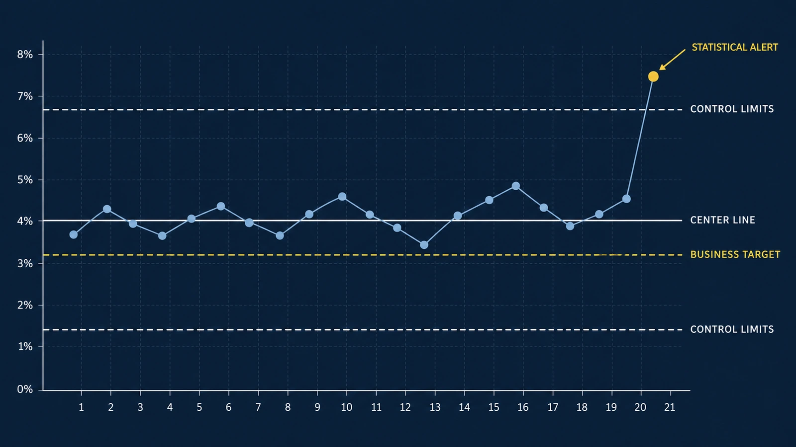
Your dashboard shows that the customer service error rate increased from 4.1% last week to 5.2% this week.
Should management investigate immediately?
Should the team change its operating procedures?
Should the result trigger an executive alert?
Or is this simply the kind of variation that occurs in an otherwise stable process?
Many business dashboards make these questions unnecessarily difficult.
They display current performance, historical averages, and business targets. Some use red and green indicators to suggest whether a result is good or bad.
But a metric moving in the wrong direction does not necessarily mean the underlying process has changed.
Similarly, a metric remaining close to its historical average does not mean the process is performing well enough.
These are two different analytical questions:
Is the process behaving differently from its established pattern?
And:
Is the process delivering the level of performance the business requires?
Statistical process control helps answer the first question.
Business targets and operational requirements help answer the second.
Understanding the distinction can make performance monitoring more useful and reduce unnecessary reactions to ordinary fluctuations.
Why Comparing This Week With Last Week Can Be Misleading
Consider an operations team processing hundreds of transactions every week.
Some transactions require corrections.
The weekly error rate naturally varies.
One week, the rate might be 3.8%.
The following week, it might be 4.6%.
The next week, it might fall to 3.9%.
A conventional dashboard may show these changes as alternating improvements and deteriorations.
But variation does not automatically indicate a meaningful process change.
Even if the underlying probability of an error remains constant, the observed proportion will fluctuate because each week's transactions are different.
This distinction matters because management decisions have consequences.
Investigating every increase consumes time.
Changing a stable process unnecessarily can introduce additional variation.
Ignoring genuine process changes can allow problems to continue.
The objective is not to eliminate investigation.
It is to make investigation more evidence-based.
Common-Cause and Special-Cause Variation
Statistical process control distinguishes between two broad categories of variation.
Common-Cause Variation
Common-cause variation describes the fluctuations inherent in an established process.
Examples may include ordinary differences in transaction complexity, customer behavior, workload, or other recurring conditions.
A process experiencing only common-cause variation may be statistically stable.
That does not mean every observation is identical.
It means the process behaves consistently with its established pattern of variation.
Special-Cause Variation
Special-cause variation refers to behavior inconsistent with the established process pattern.
Possible explanations might include:
- A software deployment
- A change in staffing
- A new operating procedure
- A reporting error
- An unusual customer population
- An equipment failure
- A change in transaction mix
These are potential explanations, not conclusions.
A statistical signal does not identify the cause.
It tells the analyst that the observed behavior deserves further investigation.
NHS Scotland's quality improvement guidance on variation emphasizes that reacting to common-cause variation as though it were a special cause can make a process worse. It also emphasizes the opposite risk: overlooking meaningful changes by treating them as ordinary variation.
The purpose of statistical process control is to help distinguish these situations.
What Is a Control Chart?
A control chart plots process measurements in chronological order.
It typically includes three statistical reference lines:
- A center line representing the established process level
- An upper control limit
- A lower control limit
These limits are estimated using an appropriate statistical model.
They describe the range of variation expected under the assumed stable-process conditions.
A point outside a control limit is a statistical signal that the process may have changed.
Additional signal rules can identify certain nonrandom patterns even when individual observations remain within the limits.
The American Society for Quality's control-chart guidance describes control charts as tools for examining process behavior over time and identifying evidence of unusual variation.
Control charts are not simply line charts with arbitrary thresholds.
The statistical assumptions and calculations matter.
Control Limits Are Not Business Targets
This distinction is fundamental.
A business target represents the performance the organization wants to achieve.
A control limit represents the variation expected from the process under the selected statistical model.
Suppose a company wants its transaction error rate below 3%.
That is a business requirement.
Now suppose the historical process averages 4.05%.
The process might consistently produce results around 4.05%, with ordinary fluctuations above and below that level.
It could be statistically stable.
But it would still be failing to achieve the business target.
A stable process is not necessarily a satisfactory process.
Similarly, a process might temporarily remain below the business target while displaying a statistical signal of deterioration.
These questions should be evaluated separately.
Worked Example: Monitoring Weekly Transaction Errors
Consider a hypothetical company that processes customer transactions.
Each transaction is classified as either:
- Completed without a recorded error
- Completed with at least one recorded error
The business wants to monitor the weekly proportion of transactions containing an error.
For simplicity, assume:
- Each transaction is counted once.
- The error definition remains consistent.
- Each transaction has a binary error outcome.
- Weekly observations represent comparable operating conditions.
- Transactions are sufficiently independent for the illustrative binomial model.
- The baseline period has no identified special-cause signals.
- The process is initially treated as having a constant underlying error probability.
These assumptions would need verification in a real implementation.
The following data is entirely hypothetical. It is not based on an actual UAD client.
Step 1: Establish the Baseline
The company has 20 weeks of historical observations. Each week contains 500 transactions.
| Week | Transactions | Transactions With Errors | Error Rate |
|---|---|---|---|
| 1 | 500 | 18 | 3.6% |
| 2 | 500 | 22 | 4.4% |
| 3 | 500 | 19 | 3.8% |
| 4 | 500 | 21 | 4.2% |
| 5 | 500 | 20 | 4.0% |
| 6 | 500 | 24 | 4.8% |
| 7 | 500 | 17 | 3.4% |
| 8 | 500 | 23 | 4.6% |
| 9 | 500 | 19 | 3.8% |
| 10 | 500 | 21 | 4.2% |
| 11 | 500 | 18 | 3.6% |
| 12 | 500 | 22 | 4.4% |
| 13 | 500 | 20 | 4.0% |
| 14 | 500 | 16 | 3.2% |
| 15 | 500 | 25 | 5.0% |
| 16 | 500 | 19 | 3.8% |
| 17 | 500 | 23 | 4.6% |
| 18 | 500 | 21 | 4.2% |
| 19 | 500 | 17 | 3.4% |
| 20 | 500 | 20 | 4.0% |
Total transactions:
20 × 500 = 10,000
Total transactions with errors:
405
Baseline error proportion:
405 / 10,000 = 0.0405
Therefore:
Baseline error rate = 4.05%.
This becomes the provisional center line of the control chart.
Before operational use, the organization should confirm that the baseline represents a reasonably stable process. A historical average calculated from a changing process may not provide meaningful control limits.
Step 2: Choose the Appropriate Control Chart
The outcome is binary at the transaction level. Each transaction either has an error or does not. The metric is the proportion of transactions with errors.
A p-chart is a conventional statistical process control method for monitoring proportions of nonconforming units. The NIST proportions control-chart reference describes the binomial model.
Under its assumptions:
p = underlying error probability
n = number of transactions in the sample
Step 3: Calculate the Control Limits
Here, p = 0.0405 and n = 500.
First calculate the estimated standard deviation:
Upper control limit:
Lower control limit:
| Reference | Error Rate |
|---|---|
| Lower control limit | 1.41% |
| Center line | 4.05% |
| Upper control limit | 6.69% |
| Business target | 3.00% |
Notice that the business target is not used to calculate the control limits.
The target is an externally defined performance requirement.
The control limits are estimated from the baseline process.
These values answer different questions.
Step 4: Interpret a New Weekly Observation
During Week 21, the company processes another 500 transactions. Of those, 38 contain an error.
Observed error rate:
38 / 500 = 0.076
Therefore:
Week 21 error rate = 7.6%.
Compare this result with the upper control limit:
7.6% > 6.69%
The observation exceeds the upper control limit.
Under the specified p-chart assumptions, this is a statistical signal.
The team should investigate.
But the chart does not tell management why the error rate increased.
The investigation should examine operational and measurement evidence.
For example:
- Was a new software version introduced?
- Did the transaction mix change?
- Were employees assigned unfamiliar tasks?
- Did the error definition change?
- Was the data extracted correctly?
The statistical result justifies investigation. It does not prove any particular explanation.
Step 5: Why Sample Size Changes the Interpretation
Now consider Week 22. Only 150 transactions were processed. Thirteen contained an error.
Observed error rate:
13 / 150 ≈ 0.0866666667
Week 22 error rate = 8.66666667%.
At first glance, this looks worse than Week 21. A dashboard ranking weeks by error rate would identify Week 22 as the worse result.
But Week 22 has a substantially smaller denominator. Smaller samples generally produce greater sampling variation in observed proportions.
For a p-chart, the control limits depend on sample size. Using p = 0.0405 and n = 150:
The observed Week 22 rate is 8.66666667%, below the sample-size-adjusted upper control limit. Under the simple single-point three-sigma rule, Week 22 does not generate an additional upper-limit signal.
| Observation | Errors | Transactions | Error Rate | Upper Control Limit | Above UCL? |
|---|---|---|---|---|---|
| Week 21 | 38 | 500 | 7.60% | 6.69% | Yes |
| Week 22 | 13 | 150 | 8.67% | 8.88% | No |
This is the central lesson.
A larger observed percentage is not necessarily stronger statistical evidence of a process change.
The denominator matters.
This does not mean Week 22 is acceptable. It remains above the business target.
It also does not erase the signal observed in Week 21. The same baseline is being used for illustration; if a process shift is confirmed, the organization should reassess the monitoring model.
A full interpretation should also consider applicable run rules and the complete time sequence.
Step 6: Translate the Statistical Result Into a Business Decision
The business target is 3% error rate. The historical process average is 4.05%.
The difference is:
4.05% − 3.00% = 1.05 percentage points
At 500 transactions per week, the expected difference is:
500 × 0.0105 = 5.25 transactions
This represents approximately 5.25 additional error-containing transactions per week relative to a hypothetical process operating at exactly 3%. The fractional result is an expected value. It does not represent a fraction of an actual transaction.
Suppose the organization estimates that each error-containing transaction generates an average of $40 in avoidable correction costs.
The illustrative weekly cost difference is:
5.25 × $40 = $210
Over 52 comparable weeks:
$210 × 52 = $10,920
The estimated annual economic difference is:
$10,920.
This calculation assumes:
- Weekly volume remains 500
- The error-rate difference persists
- The $40 cost estimate is appropriate
- Costs scale approximately with the number of errors
- No additional relevant costs or benefits are omitted
It is a hypothetical planning calculation. It is not evidence that a specific intervention would save $10,920.
Achieving the target may require investment, and that investment has its own costs and uncertainty.
The calculation helps quantify the value of the performance gap. It does not establish how to close it.
Four Different Management Situations
Combining process stability with business performance creates four useful management situations.
| Process Behavior | Business Target | Interpretation | Appropriate Response |
|---|---|---|---|
| Stable | Met | Predictable and acceptable under the defined criteria | Continue monitoring |
| Stable | Missed | Predictably underperforming | Redesign or improve the underlying process |
| Statistical signal | Met | Performance may have changed despite meeting target | Investigate the signal |
| Statistical signal | Missed | Potential process change and unacceptable performance | Investigate promptly and assess corrective action |
This framework prevents two common mistakes.
The first is treating every unfavorable fluctuation as a crisis.
The second is treating a stable but inadequate process as satisfactory.
Stability and performance are different dimensions.
Both matter.
What Should Trigger a Dashboard Alert?
A conventional dashboard might trigger an alert whenever the error rate exceeds 5%. That is easy to implement.
But why 5%?
If the threshold has no relationship to process behavior or business requirements, the alert may create unnecessary noise.
A stronger monitoring design separates several alert types.
Statistical Signal
An observation exceeds an appropriate control limit or meets a predefined statistical signal rule.
Purpose: Identify behavior inconsistent with the established process model.
Business Target Violation
The observed performance fails an agreed business requirement.
Purpose: Identify an unacceptable outcome.
Data Quality Alert
The metric may be unreliable because of missing records, delayed data, duplicate observations, or changed definitions.
Purpose: Prevent management from acting on invalid information.
Operational Escalation
A predefined combination of evidence indicates that a manager should intervene.
Purpose: Connect measurement to a concrete operational decision.
These alerts may overlap.
But they should not be treated as interchangeable.
A statistical signal is not automatically a business emergency.
A target violation is not automatically evidence of a process change.
A data quality failure may invalidate both interpretations.
Control Charts Do Not Establish Causality
Suppose the company introduces a new training program. The error rate subsequently declines. The control chart eventually identifies a sustained downward shift.
Can management conclude that the training caused the improvement?
Not from the control chart alone.
The chart may provide evidence that process behavior changed. It does not establish which intervention caused that change.
Other explanations may include:
- Changes in customer mix
- Different staffing levels
- New software
- Reduced transaction complexity
- Revised error definitions
- Seasonal effects
- Concurrent process improvements
A stronger causal evaluation may require a comparison group, randomized rollout, interrupted time-series design, or another appropriate study design.
The control chart answers: “Has the process shown evidence of a change?”
Causal analysis asks: “What caused the change?”
Those questions are related but distinct.
Choosing the Right Control Chart
Not every KPI should use a p-chart. The appropriate method depends on the measurement structure.
| Data Structure | Possible Chart | Example |
|---|---|---|
| Proportion of units with a binary outcome | p-chart | Percentage of orders with an error |
| Number of nonconforming units with fixed sample size | np-chart | Defective items in batches of equal size |
| Count of events over constant opportunity | c-chart | Defects per standardized inspection unit |
| Event rate with varying exposure | u-chart | Defects per unit when inspection opportunities vary |
| Individual continuous measurements | Individuals and moving-range chart | Daily processing time |
| Subgroup averages and variation | X-bar and R/S charts | Average processing time from repeated samples |
The chart type should follow the data-generating process.
For example, counting the number of customers who experience at least one error is different from counting the total number of errors.
One customer may experience several errors.
A p-chart for the proportion of affected customers is not interchangeable with a chart for errors per transaction.
The distinction affects both the numerator and the statistical model.
Important Statistical Limitations
Control charts are useful, but their assumptions deserve attention.
Independence
The illustrative p-chart assumes transactions are sufficiently independent. If errors occur in clusters, the observed variability may differ from the binomial model. For example, a temporary software defect might affect many consecutive transactions. Ignoring clustering can produce misleading control limits.
Stable Baseline
Control limits should be based on a reasonably stable reference process. If the baseline contains substantial changes in operating conditions, a single average may not represent one coherent process.
Changing Case Mix
A hospital, service center, or business unit may handle different types of cases over time. If the proportion of difficult cases increases, the overall error rate may change even if performance within each case category remains constant. Risk adjustment or stratification may be necessary.
Seasonality and Autocorrelation
Weekly observations may be correlated. Seasonal patterns can also affect performance. Standard control charts may produce misleading signals when these dependencies are ignored. More appropriate time-series or risk-adjusted methods may be required.
Multiple Signal Rules
A single three-sigma limit is not the only way to identify unusual behavior. Run and trend rules can detect certain patterns. However, using more rules generally increases sensitivity and may also increase false alarms. Organizations should define their monitoring rules in advance and evaluate the consequences of unnecessary investigations.
Baseline Uncertainty
The baseline rate is estimated from historical data. It is not known perfectly. The resulting control limits are therefore estimates. Twenty historical observations can provide a practical starting point, but they do not guarantee a valid model. The amount of data required depends on the chart, process, assumptions, and intended use.
How to Implement Control Charts in Power BI or Tableau
A practical implementation begins with a reliable analytical dataset.
For a weekly transaction error-rate chart, the dataset should contain:
- Reporting week
- Number of eligible transactions
- Number of transactions with errors
- Error proportion
- Baseline process estimate
- Appropriate upper control limit
- Appropriate lower control limit
- Business target
- Data completeness status
The error rate is:
Error Rate = Error Transactions / Eligible Transactions
For a p-chart with changing sample sizes, the limits should be calculated using the corresponding denominator. The dashboard should not apply one fixed p-chart limit to every period when denominators vary materially.
The visualization can then display:
- Weekly error rate
- Baseline center line
- Upper control limit
- Lower control limit
- A separately identified business target
Use different visual treatments for statistical limits and management targets. The purpose is to prevent users from confusing expected process behavior with acceptable performance.
A useful dashboard may also allow users to inspect:
- Transaction volume
- Location
- Department
- Customer segment
- Product category
- Operational changes
- Known data-quality incidents
These diagnostic dimensions help investigate statistical signals. They do not automatically establish causality.
For a broader discussion of connecting metrics to decisions, see UAD Consulting's article on building a KPI framework.
For related visualization principles, see the article on how data visualization supports better business decisions.
Organizations seeking help with implementation can explore UAD Consulting's business intelligence and data visualization services.
A Practical Investigation Workflow
When a statistical signal appears, management should follow a consistent investigation process.
First: Verify the Measurement
Check:
- Data completeness
- Reporting period
- Numerator and denominator definitions
- Duplicate records
- Source-system changes
- Calculation logic
A broken pipeline can produce an apparent process change.
Second: Verify the Statistical Signal
Confirm:
- Correct chart type
- Appropriate baseline
- Correct denominator
- Valid control limits
- Relevant signal rules
- Reasonable assumptions
Third: Review Operational Context
Investigate events that could explain the change. Document software releases, staffing changes, workflow changes, demand shifts, policy changes, and exceptional operating conditions.
Fourth: Determine the Appropriate Action
A signal may justify additional analysis, immediate containment, process review, targeted operational intervention, or a controlled improvement experiment.
The response should reflect the severity and business consequences of the problem.
Fifth: Evaluate the Result
Continue monitoring after an intervention. If the process changes and establishes a new stable operating pattern, consider whether a new baseline is justified.
Do not automatically recalculate control limits after every unusual observation. That can conceal meaningful changes.
Frequently Asked Questions
What Is the Difference Between a KPI Target and a Control Limit?
A KPI target represents desired performance. A control limit is calculated from process behavior using a statistical model. A process can remain within its control limits while consistently missing its business target.
Does a Point Outside the Control Limits Prove Something Went Wrong?
No. It provides a statistical signal that deserves investigation. The chart does not identify the cause, and false signals are possible.
Can a Process Be Stable but Perform Poorly?
Yes. A process can behave predictably while consistently failing to meet its required performance level. Improving such a process may require changing its underlying design rather than reacting to individual observations.
Why Do Control Limits Change With Sample Size?
For proportions, sampling variability depends on the denominator. Smaller samples generally produce more variable observed proportions. A p-chart accounts for this through sample-size-dependent control limits.
Can Control Charts Be Used Outside Manufacturing?
Yes. The underlying methods can support monitoring in healthcare, customer service, finance, operations, and other settings. The statistical model must still fit the measurement process.
Can a Control Chart Prove an Intervention Worked?
No. A control chart can identify evidence of a process shift. Attributing that shift to a particular intervention requires additional evidence and an appropriate causal evaluation.
Better Dashboards Distinguish Change From Noise
A dashboard should do more than display whether a KPI increased or decreased.
It should help decision-makers understand what the observed movement means.
Statistical process control provides a structured way to distinguish ordinary process variation from signals that warrant investigation.
Business targets establish whether the observed performance is acceptable.
Data-quality controls establish whether the measurement can be trusted.
Causal analysis helps determine whether an intervention produced a change.
These are complementary analytical responsibilities.
The practical sequence is:
Validate the Data → Understand Process Variation → Compare With Business Requirements → Investigate Signals → Evaluate Causes → Decide on Action
The goal is not to eliminate variation.
It is to distinguish the variation that requires action from the variation that does not.
That distinction can make performance monitoring more reliable, management discussions more productive, and operational decisions more defensible.
References and Further Reading
Turn KPI Monitoring Into Better Decisions
UAD Consulting helps organizations develop clearer performance measures, analytical dashboards, and decision-focused reporting systems. From KPI design to statistical analysis and business intelligence, the goal is to distinguish meaningful changes from ordinary variation and connect evidence to action.
Explore ServicesGet in Touch