Imagine that your company conducts a customer satisfaction survey.
The results look encouraging.
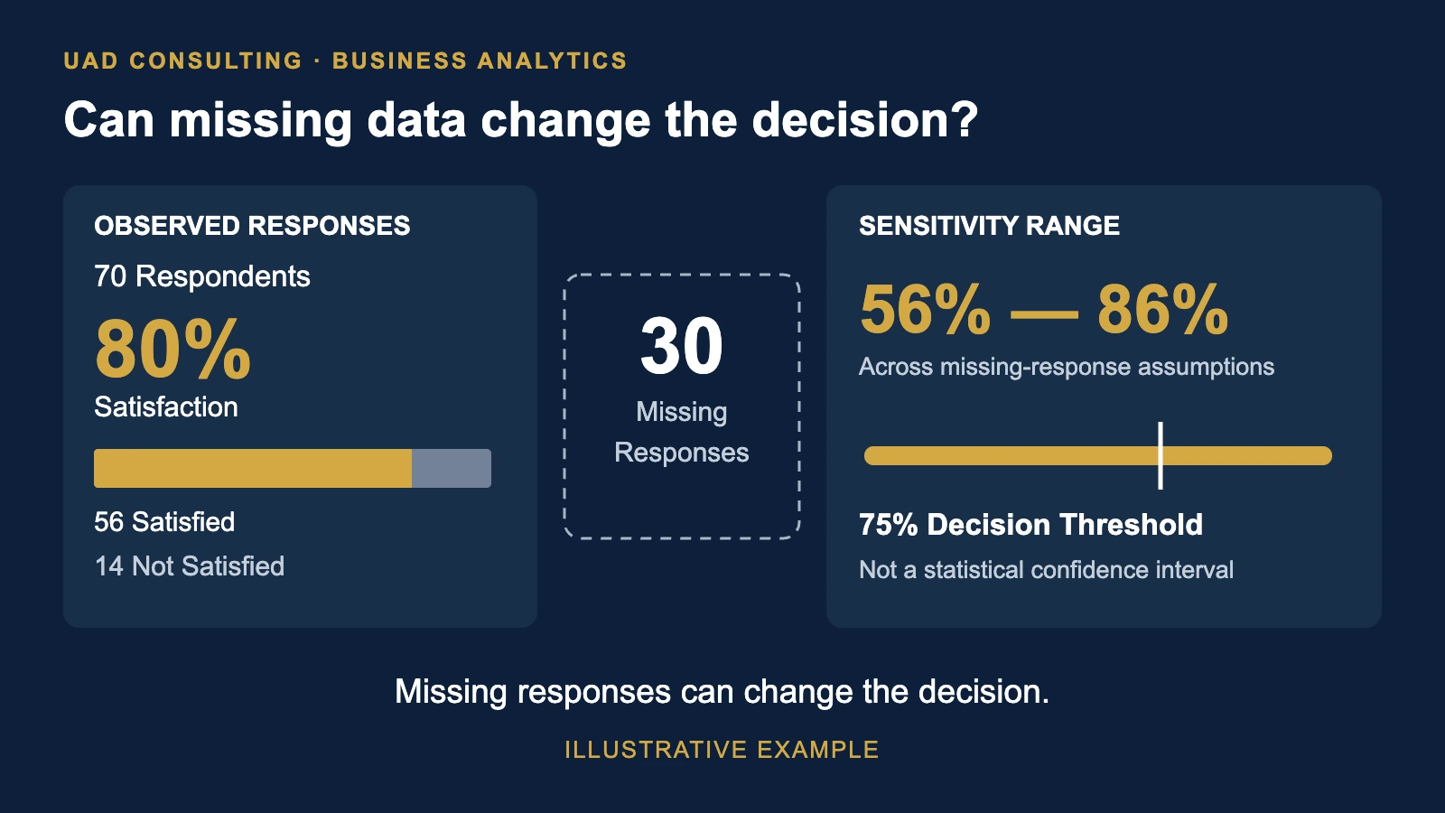
Among customers who responded, 80% report being satisfied.
Management considers this a strong result and begins planning an expansion of the service.
But there is an important detail.
Only 70% of the customers invited to participate completed the survey.
The remaining 30% never responded.
Does the reported 80% satisfaction rate accurately describe the customers who were invited?
Not necessarily.
If satisfied customers were more likely to respond than dissatisfied customers, the observed survey result could overstate satisfaction.
If dissatisfied customers were more motivated to respond, the opposite could occur.
The difficulty is that the missing responses are not observed.
Their absence creates uncertainty that cannot be eliminated simply by calculating an average.
This is the central challenge of missing-data analysis.
A dataset can contain correct calculations, valid records, and professionally designed dashboards while still producing misleading conclusions because some observations are missing.
The important question is not merely how many values are missing.
It is whether the missing values could change the decision.
The Short Answer: Missing Data Can Change Both the Estimate and the Decision
Missing data can distort an analytical result when the observed records differ systematically from the records that are missing.
For example, suppose a survey has a response rate of 70%.
Among respondents, satisfaction is 80%.
That establishes the satisfaction rate among respondents.
It does not automatically establish the satisfaction rate among all invited customers.
The overall result depends partly on the satisfaction levels of customers who did not respond.
If their outcomes differ from those of respondents, extrapolating the observed 80% to everyone may be misleading.
The same problem can arise in business and healthcare datasets when:
- Dissatisfied customers are less likely to complete surveys.
- Customers who cancel subscriptions stop reporting usage.
- High-cost healthcare encounters are more likely to have incomplete financial information.
- Marketing conversions cannot be linked to identifiable customers.
- Certain operational failures are recorded inconsistently.
- Missing values depend on customer behavior or system processes.
Different missing-data mechanisms require different analytical responses.
There is no universally correct replacement value.
A Worked Example: The Survey That Reported 80% Satisfaction
Consider a hypothetical company evaluating a premium customer-support service.
Management plans to expand the service if customer satisfaction reaches at least 75%.
The company invites 100 customers to complete a satisfaction survey.
The results are:
| Measure | Customers |
|---|---|
| Customers invited | 100 |
| Customers responding | 70 |
| Satisfied respondents | 56 |
| Dissatisfied respondents | 14 |
| Customers not responding | 30 |
The observed satisfaction rate among respondents is:
The response rate is:
These are both valid calculations.
But they describe different things.
The first measures satisfaction among respondents.
The second measures survey participation.
Neither directly identifies satisfaction among the 30 customers who did not respond.
If management interprets the observed 80% as the satisfaction rate of all 100 invited customers, it is implicitly making an assumption about the missing responses.
That assumption should be examined.
What Happens If We Replace Missing Values With the Average?
A common approach to missing numerical data is mean imputation.
The analyst calculates the average of observed values and substitutes that average for missing observations.
For a binary satisfaction indicator:
Satisfied = 1
Not satisfied = 0
The observed mean is:
Mean imputation would assign 0.80 to each of the 30 missing observations.
The resulting sum of satisfaction values becomes:
56 + (30 × 0.80)
= 80
The imputed average across all 100 records is:
The result looks complete.
The dataset now has 100 nonmissing satisfaction values.
But the information has not improved in the way the completed dataset might suggest.
The 30 missing values were replaced with an assumption derived from the 70 observed responses.
No additional customer satisfaction outcomes were measured.
The imputed values are not actual binary responses.
More importantly, this approach effectively assumes that the average satisfaction level among nonrespondents is the same as among respondents.
That assumption may be inappropriate.
Simple mean imputation can also understate variability and distort relationships between variables.
Replacing missing observations with a single estimated value should not be confused with recovering the information that was never observed.
A Sensitivity Analysis: What If Nonrespondents Are Less Satisfied?
Instead of assuming that nonrespondents have the same satisfaction rate as respondents, consider several possible values.
Let:
q = satisfaction proportion among nonrespondents
The satisfaction proportion among the 100 invited customers would be:
Overall Satisfaction =
(56 + 30q) / 100
The 56 represents known satisfied respondents.
The 30q represents the assumed number of satisfied customers among nonrespondents.
Now evaluate several scenarios.
| Assumed Satisfaction Among Nonrespondents | Estimated Satisfaction Among All Invited Customers |
|---|---|
| 0% | 56% |
| 20% | 62% |
| 40% | 68% |
| 60% | 74% |
| 80% | 80% |
| 100% | 86% |
These values are mathematically derived from the hypothetical survey.
They are not empirical estimates of actual nonrespondent satisfaction.
The table demonstrates how much the overall result depends on the missing observations.
If nonrespondent satisfaction is 80%, the overall rate is 80%.
If nonrespondent satisfaction is 40%, the overall rate is 68%.
The difference is:
A dashboard that simply fills missing observations with the respondent average would not reveal this uncertainty.
A sensitivity analysis makes the assumption visible.
The Decision Can Reverse Without Changing Any Observed Response
Return to management's decision rule.
The company plans to expand the service if satisfaction among the invited customers reaches at least 75%.
Using only the observed respondent satisfaction rate:
Management might conclude that the requirement has been met.
But suppose nonrespondent satisfaction is 40%.
The estimated overall rate becomes:
(56 + 30 × 0.40) / 100
= 68%
Under that scenario:
68% < 75%
The decision changes.
The observed survey responses have not changed.
The decision changes because the assumption about missing observations changes.
We can calculate the exact assumption required to meet the 75% threshold.
Set:
(56 + 30q) / 100 = 0.75
Multiply both sides by 100:
Subtract 56:
Therefore:
q = 19 / 30
q ≈ 63.3%
At least 19 of the 30 nonrespondents would need to be satisfied for the invited-customer satisfaction rate to reach 75%.
That is the decision boundary.
The company does not necessarily need to know the exact satisfaction rate of every nonrespondent before making any decision.
But it should understand which assumptions would support or reverse its preferred action.
This is one reason sensitivity analysis is useful.
It connects missing-data uncertainty directly to business decisions.
What Are MCAR, MAR, and MNAR?
Statisticians commonly distinguish three missing-data mechanisms.
These terms describe how the probability of missingness relates to observed and unobserved information.
They are not interchangeable.
Missing Completely at Random (MCAR)
Data are missing completely at random when the probability that a value is missing does not depend on observed or unobserved data values.
For example, suppose a random technical failure prevents a small subset of survey responses from being saved.
If the failure is genuinely unrelated to customer characteristics, satisfaction, and other relevant variables, MCAR may be plausible.
Under MCAR, complete-case analysis can provide unbiased estimates for many common targets, although excluding records generally reduces precision.
However, MCAR should not be assumed simply because a missingness pattern appears irregular.
Missing at Random (MAR)
Missing at random means that, conditional on appropriate observed information, missingness does not depend on the unobserved value itself.
The name can be confusing.
MAR does not mean missing values are randomly scattered throughout the dataset.
For example, suppose younger customers are less likely to complete a survey.
Age is recorded for every invited customer.
If response probability depends on age but, within comparable age groups, does not additionally depend on unobserved satisfaction, MAR may be a reasonable assumption conditional on age.
Methods using the observed age information may help address the missingness.
The plausibility of MAR depends on whether the relevant predictors of missingness and outcomes have been measured and appropriately modeled.
It is an assumption, not something automatically established by the data.
Missing Not at Random (MNAR)
Missing not at random occurs when missingness depends on unobserved values, even after accounting for relevant observed information.
Suppose customers with particularly negative experiences are less likely to answer the satisfaction question.
If this dependence remains after conditioning on observed customer characteristics, the missingness mechanism is MNAR.
In this situation, the observed responses may not adequately represent the missing responses.
Standard methods relying on MAR may produce misleading estimates.
Sensitivity analysis, additional data collection, and models that explicitly consider nonignorable missingness may be necessary.
Comparing the Three Mechanisms
| Mechanism | Missingness Depends On | Example |
|---|---|---|
| MCAR | Neither observed nor unobserved values | Truly random data loss |
| MAR | Observed variables, after appropriate conditioning | Response differs by recorded customer age |
| MNAR | Unobserved values after conditioning | Satisfaction itself influences nonresponse |
These are conceptual examples.
Real missingness mechanisms can be difficult to establish.
A dataset generally cannot prove the absence of MNAR solely from the observed values.
The analyst must combine statistical diagnostics with knowledge of the data collection process.
For a detailed methodological treatment, see Sterne and colleagues' BMJ article on multiple imputation and missing-data assumptions.
Why Missingness Percentage Alone Is Not Enough
Suppose two datasets each have 10% missing values.
Dataset A has missing values caused by a genuinely random system failure.
Dataset B has missing values concentrated among customers who experienced serious service problems.
Both have 90% completeness.
But the potential analytical consequences are different.
Dataset A may lose statistical precision without introducing substantial systematic bias under the relevant assumptions.
Dataset B may systematically misrepresent customer satisfaction.
A simple data-quality dashboard might report both datasets as 90% complete.
That number does not describe the missingness mechanism.
This is why completeness checks should be interpreted alongside the analytical question.
For a broader framework, see UAD Consulting's article on data-quality checks for analytics pipelines.
The central distinction is:
Completeness measures how much information is recorded.
Missing-data analysis asks what the missing information may imply for the result.
Complete-Case Analysis Is Not Always Wrong
Complete-case analysis uses only observations with the required variables available.
It is simple, transparent, and sometimes appropriate.
However, excluding incomplete records can reduce sample size and statistical precision.
It can also introduce selection bias.
The direction and magnitude of bias depend on the missingness mechanism, the estimand, and the analysis being performed.
For example, if survey participation depends on satisfaction, analyzing respondents alone may produce a biased estimate of satisfaction among all invited customers.
But if missingness is unrelated to the outcome under suitable conditions, a complete-case estimate may remain unbiased for a particular target.
Therefore, the correct conclusion is not:
"Never use complete-case analysis."
It is:
"Do not assume complete-case analysis is unbiased without examining why observations are missing."
This distinction also matters when evaluating sample size.
A large dataset does not automatically solve selection bias.
See our guide on sample size and business decisions for the difference between precision, representativeness, and decision relevance.
When Is Multiple Imputation More Appropriate?
Multiple imputation is a statistical approach that generates several plausible completed datasets rather than relying on one fixed replacement value.
The procedure generally involves:
- Modeling missing values using appropriate observed information.
- Generating multiple completed datasets.
- Performing the intended analysis separately in each dataset.
- Combining estimates and uncertainty using appropriate pooling rules.
The objective is not to discover the actual missing observations.
It is to account for uncertainty about them under an explicit statistical model.
Multiple imputation can be useful when MAR is plausible and the imputation model appropriately represents relationships relevant to the analysis.
However, it does not automatically solve MNAR.
It also requires attention to model specification, variable types, interactions, analysis compatibility, and uncertainty.
For a clinical or economic analysis, using multiple imputation without examining the assumptions may create a false impression of methodological rigor.
Sterne and colleagues discuss both the potential benefits and the pitfalls of multiple imputation in epidemiological and clinical research.
Missing Values in Machine Learning Require a Different Perspective
Missing-data handling also matters in predictive modeling.
A machine-learning system may use mean, median, or most-frequent-value imputation to construct a usable feature matrix.
This can be operationally reasonable.
The purpose is often to generate predictions, not to estimate a population mean or causal effect.
For example, a customer-churn model might use account age, purchase frequency, customer support interactions, and subscription activity.
If purchase frequency is missing for some customers, a preprocessing pipeline may impute a value and include an indicator showing that the original value was missing.
The missingness indicator may itself contain predictive information.
However, several safeguards matter.
First, preprocessing statistics should be learned using training data only.
Calculating imputation values using the entire dataset before train/test separation can leak information from evaluation data into model development.
Second, the same fitted transformation must be applied consistently to validation, test, and production observations.
Third, the imputation method should be evaluated based on the intended predictive task.
A method that produces acceptable predictive performance does not necessarily produce unbiased population estimates.
Fourth, a missingness indicator is not proof that the underlying missingness mechanism has been understood.
Scikit-learn's SimpleImputer documentation describes mean, median, most-frequent, constant-value, and missing-indicator options.
The appropriate method depends on the analytical objective.
Reproduce the Sensitivity Analysis in BigQuery
The hypothetical customer satisfaction example can be reproduced using GoogleSQL in BigQuery.
The following query uses synthetic values defined inside the query.
It does not require access to a customer database.
WITH survey AS (

  SELECT
    100 AS invited_customers,
    70 AS responding_customers,
    56 AS satisfied_respondents,
    0.75 AS decision_threshold

),

assumptions AS (

  SELECT assumed_nonrespondent_satisfaction

  FROM UNNEST([
    0.0,
    0.2,
    0.4,
    0.6,
    0.8,
    1.0
  ]) AS assumed_nonrespondent_satisfaction

)

SELECT

  a.assumed_nonrespondent_satisfaction,

  ROUND(
    100 * SAFE_DIVIDE(
      s.satisfied_respondents,
      s.responding_customers
    ),
    1
  ) AS respondent_satisfaction_pct,

  ROUND(
    100 * SAFE_DIVIDE(
      s.satisfied_respondents
      +
      (
        s.invited_customers
        -
        s.responding_customers
      )
      *
      a.assumed_nonrespondent_satisfaction,

      s.invited_customers
    ),
    1
  ) AS invited_cohort_satisfaction_pct,

  CASE

    WHEN SAFE_DIVIDE(
      s.satisfied_respondents
      +
      (
        s.invited_customers
        -
        s.responding_customers
      )
      *
      a.assumed_nonrespondent_satisfaction,

      s.invited_customers
    ) >= s.decision_threshold

    THEN 'Meets threshold'

    ELSE 'Below threshold'

  END AS decision_result

FROM survey s

CROSS JOIN assumptions a

ORDER BY
  a.assumed_nonrespondent_satisfaction;
Expected results:
| Nonrespondent Satisfaction Assumption | Respondent Satisfaction | Invited-Cohort Satisfaction | Decision |
|---|---|---|---|
| 0% | 80% | 56% | Below threshold |
| 20% | 80% | 62% | Below threshold |
| 40% | 80% | 68% | Below threshold |
| 60% | 80% | 74% | Below threshold |
| 80% | 80% | 80% | Meets threshold |
| 100% | 80% | 86% | Meets threshold |
The query demonstrates a sensitivity analysis.
It does not estimate which assumption is most likely to be true.
That requires additional evidence or modeling assumptions.
It also does not establish statistical confidence intervals.
The values are conditional scenario calculations.
The distinction matters.
A sensitivity range describes how conclusions change across assumptions.
A confidence interval generally describes uncertainty under a specified statistical sampling model.
They should not be presented as interchangeable.
What Can We Learn From the Best- and Worst-Case Bounds?
In the hypothetical example, 56 customers are known to be satisfied.
There are 30 missing responses.
If every nonrespondent is dissatisfied:
Overall invited-cohort satisfaction = 56%
If every nonrespondent is satisfied:
Overall invited-cohort satisfaction = 86%
Therefore, without additional restrictions, the invited-cohort satisfaction proportion lies between:
56% and 86%
These are identification bounds for the finite group of 100 invited customers, assuming the recorded responses are accurate and satisfaction is binary.
They are not a 95% confidence interval.
They are also not necessarily bounds for the satisfaction rate of the company's entire customer population.
That broader inference would require considering how the 100 invited customers were selected.
The bounds may be wide, but they communicate something important.
The observed information alone is insufficient to determine whether the 75% decision threshold has been met.
Additional information could narrow the uncertainty.
How Can a Business Reduce Missing-Data Uncertainty?
The most useful intervention may be improving data collection rather than selecting a more sophisticated imputation algorithm.
For a customer satisfaction survey, the business could investigate:
- Whether survey invitations were delivered successfully.
- Whether response rates differ by customer segment.
- Whether dissatisfied customers are more likely to stop participating.
- Whether some devices or browsers prevent survey completion.
- Whether customers with recent support escalations respond differently.
- Whether nonrespondents can be contacted through a follow-up survey.
Observed customer characteristics may help evaluate whether respondents and nonrespondents differ.
A follow-up sample of nonrespondents can provide additional evidence.
However, follow-up respondents may still differ from customers who remain unreachable.
The organization should not assume that a second survey automatically eliminates nonresponse bias.
A stronger design would consider how the follow-up sample was selected, how responses were collected, and whether remaining nonresponse could still affect the result.
Applications Beyond Customer Satisfaction
Missing-data sensitivity analysis is relevant across several business domains.
Healthcare Analytics
Healthcare administrative and clinical datasets may contain missing cost, outcome, severity, or utilization information.
For example, if encounters with unusually high treatment costs are more likely to have missing financial values, imputing missing costs using the overall observed mean may underestimate total cost.
That is a possible mechanism, not a universal pattern.
The analyst should investigate missingness by facility, encounter type, patient characteristics, and other relevant factors.
The correct method depends on the study design, estimand, data structure, and plausible missingness mechanism.
Marketing Analytics
Marketing attribution datasets may not connect every conversion to a known advertising interaction.
The observed conversions can be accurately counted while attribution coverage remains incomplete.
However, missing attribution information should not automatically be interpreted as missing conversions.
These are different measurement problems.
The analyst should distinguish whether an outcome is missing, an identifier is missing, or the relationship between records cannot be established.
Operations Analytics
Equipment downtime may be underreported when maintenance logs are completed inconsistently.
If the most disruptive failures are also the least likely to be recorded accurately, observed downtime statistics may understate operational risk.
Customer Retention
A subscription dataset may contain missing cancellation reasons.
Analyzing only customers who provided a reason may misrepresent why customers leave if reason reporting depends on the customer's experience.
Across these settings, the same principle applies.
The missingness mechanism matters because the observed population may not represent the population relevant to the decision.
A Decision-Oriented Missing-Data Framework
Before replacing missing values, a business should answer six questions.
1. What Decision Depends on the Data?
Identify the action.
For example:
Expand the service if satisfaction reaches 75%.
A decision threshold helps determine which uncertainties matter.
2. What Is the Target Quantity?
Define the estimand.
Are we estimating satisfaction among respondents?
Among all invited customers?
Among all active customers?
Or among a broader market?
These are different populations.
The available data may support some estimates more directly than others.
3. What Is Missing?
Distinguish missing outcomes, predictors, identifiers, timestamps, entire records, and unobserved relationships.
These problems are not equivalent.
4. Why Might the Data Be Missing?
Investigate the data collection process.
Compare observed characteristics of complete and incomplete records.
Consider MCAR, MAR, and MNAR.
Document which assumptions are plausible and which remain uncertain.
5. Could Reasonable Assumptions Reverse the Decision?
Calculate sensitivity scenarios.
Where possible, identify the assumption required to cross the decision threshold.
In our example, the relevant boundary was approximately 63.3% satisfaction among nonrespondents.
6. What Additional Evidence Would Be Valuable?
Consider whether collecting more information, improving measurement, or applying a defensible statistical model could change the decision.
If every plausible assumption supports the same action, additional data may have limited decision value.
If reasonable assumptions produce opposite decisions, the uncertainty deserves greater attention.
This connects missing-data analysis with a broader decision-analytics principle:
The value of information depends on whether it can improve the decision, not merely whether it increases the number of available observations.
Does Missing Data Prove That a Business Result Is Biased?
No.
Missing data create a potential source of bias.
They do not automatically establish the direction or magnitude of that bias.
In our example, nonrespondents could be less satisfied, equally satisfied, or more satisfied than respondents.
Without additional evidence, the analyst should not claim to know which scenario is correct.
Likewise, an association between survey nonresponse and customer churn does not prove that dissatisfaction caused nonresponse.
The relationship could reflect other factors, including customer engagement, contact preferences, survey accessibility, or unmeasured characteristics.
Correlation is not causation.
An imputation model can estimate missing values under assumptions, but it does not establish the causal reason observations were missing.
The appropriate conclusion should reflect what the data and assumptions actually support.
Frequently Asked Questions
Is mean imputation always wrong?
No.
Mean imputation can be a practical preprocessing choice for some predictive workflows.
However, it can distort variability, relationships, and inferential uncertainty.
It should not be treated as a universally valid solution for estimating population characteristics.
Does 30% missing data make a dataset unusable?
Not automatically.
The consequences depend on the missingness mechanism, analytical objective, sample size, available auxiliary information, and the sensitivity of the decision.
A smaller amount of systematically missing data can sometimes be more problematic than a larger amount of plausibly random missingness.
Can multiple imputation solve MNAR?
Not automatically.
Conventional multiple imputation often relies on MAR assumptions.
MNAR requires additional assumptions, models, or sensitivity analyses.
Can we prove that data are MAR?
Generally, MAR cannot be established solely from the observed dataset.
Its plausibility depends on substantive knowledge and assumptions about the missingness process.
What is the difference between missing-data bounds and confidence intervals?
Missing-data bounds describe values consistent with specified information and assumptions.
Confidence intervals describe sampling uncertainty under a statistical model.
They answer different questions.
Should missingness be shown in a dashboard?
For decision-relevant metrics, reporting completeness, denominators, and missingness by important segment can be useful.
A dashboard should not present an imputed estimate as though every underlying outcome was observed.
The Better Question Is Not "How Do We Fill the Missing Values?"
Return to the customer satisfaction survey.
Among respondents, satisfaction was 80%.
But 30% of invited customers did not respond.
The observed information allowed satisfaction among all invited customers to range from 56% to 86%.
The company's expansion threshold was 75%.
Under one assumption, expansion appeared justified.
Under another, the threshold was not met.
The calculation was never the central problem.
The problem was deciding what could reasonably be inferred from incomplete information.
Replacing missing values with an average can make a dataset look complete.
It cannot make unobserved outcomes known.
A more defensible analytical process makes assumptions explicit, evaluates how conclusions change, and connects uncertainty to the decision.
The objective is not to produce the cleanest-looking dataset.
It is to understand what the available evidence can support.
References and Further Reading
- Sterne, J. A. C., White, I. R., Carlin, J. B., Spratt, M., Royston, P., Kenward, M. G., Wood, A. M., and Carpenter, J. R. (2009). Multiple imputation for missing data in epidemiological and clinical research: potential and pitfalls. BMJ, 338, b2393. DOI: 10.1136/bmj.b2393.
- Missing Data in Clinical Studies: Issues and Methods. Peer-reviewed methodological review available through PubMed Central. PMC3948388.
- Scikit-learn. SimpleImputer documentation. Official documentation covering simple imputation strategies and missingness indicators.
All numerical examples in this article are hypothetical.
They are intended to demonstrate analytical principles, not to report empirical findings about a real company.
Make Better Decisions With Incomplete Data
UAD Consulting helps organizations evaluate data quality, statistical assumptions, business metrics, and analytical uncertainty before turning results into decisions.
Whether the challenge involves incomplete customer information, missing healthcare costs, unreliable reporting, or analytical modeling, the goal is to connect available evidence with defensible business decisions.
Explore our Business Analytics & Reporting services to discuss an analytical question or data-quality challenge.
Explore ServicesGet in Touch