A hospital introduces a new care-management program.
The program is designed to provide additional monitoring and follow-up services to eligible patients.
Several months later, the analytics team evaluates patient outcomes.
The initial results look promising.
Patients who participated in the program experienced fewer deaths than patients who never participated.
Management interprets the difference as evidence that the program improved survival.
But there is an important question:
When did patients actually enter the program?
Some patients enrolled immediately.
Others enrolled several weeks after becoming eligible.
Meanwhile, some patients died before they had an opportunity to enroll.
If the analysis classifies patients according to whether they ever participated in the program, it may unintentionally create an advantage for the participant group.
To become a participant, a patient first had to survive long enough to enter the program.
That required survival period can distort the comparison.
This problem is known as immortal time bias.
It is a well-established methodological concern in observational healthcare research.
The problem is especially relevant when analysts use electronic health records, insurance claims, or administrative healthcare datasets to evaluate treatments and programs that begin after the start of follow-up.
The central lesson is straightforward:
A patient should not be classified as exposed to an intervention during a period when the intervention had not yet begun.
What Is Immortal Time Bias?
Immortal time bias occurs when the design or analysis of an observational study incorrectly handles a period during which an individual must remain event-free to qualify for a particular exposure group.
The word "immortal" is statistical terminology.
It does not mean that a patient is literally unable to die.
Instead, it describes a period during which the outcome cannot occur among individuals classified into a group using future information.
Consider a patient who enters a healthcare cohort on January 1.
The patient begins a treatment on January 31.
Suppose the study classifies this patient as treated from January 1 because the patient eventually received treatment.
The classification creates a problem.
To receive treatment on January 31, the patient had to survive until that date.
A patient who died on January 10 could not subsequently begin treatment on January 31.
Therefore, the eventual treatment group is selected partly on the basis of survival before treatment.
If the analysis attributes those first 30 days to the treated group, it incorrectly assigns untreated follow-up time to treatment exposure.
The result can make the treatment appear protective even when the apparent benefit is partly or entirely caused by the study design.
Research by Suissa demonstrated how this problem can substantially distort observational estimates of medication effectiveness.
The issue is not necessarily an error in the underlying medical records.
It can arise even when every recorded date and clinical event is correct.
The problem is how the records are used to construct the analytical comparison.
The Three Dates Every Analyst Must Distinguish
A healthcare outcomes analysis should distinguish at least three concepts.
1. Cohort Entry Date
This is the date when a patient first becomes eligible for the study.
For example:
Hospital discharge.
Diagnosis.
Enrollment in an insurance plan.
Eligibility for a care-management program.
The appropriate starting point depends on the research question.
2. Treatment Initiation Date
This is the date when the patient actually begins receiving the intervention.
Treatment initiation may occur immediately or after a delay.
For some patients, treatment may never begin.
3. Outcome or Censoring Date
This is the date when the outcome occurs or observation ends.
Examples include:
Death.
Hospital readmission.
Disease recurrence.
End of insurance coverage.
End of the study period.
Loss to follow-up.
These dates should not be treated as interchangeable.
If treatment begins after cohort entry, the period before treatment initiation requires appropriate handling.
The correct approach depends on the causal question and study design.
A Worked Example: Six Patients in a Care-Management Program
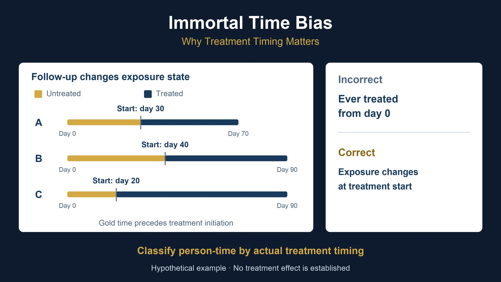
Consider a hypothetical hospital evaluating a new care-management program.
Six patients become eligible on day zero.
The hospital follows each patient for up to 90 days.
Three patients eventually enroll in the program.
Three never enroll.
The outcome of interest is death during follow-up.
The following dataset is entirely synthetic.
It does not represent actual patients or clinical findings.
| Patient | Program Start | Follow-Up Ends | Outcome |
|---|---|---|---|
| A | Day 30 | Day 70 | Death |
| B | Day 40 | Day 90 | Alive |
| C | Day 20 | Day 90 | Alive |
| D | Never | Day 10 | Death |
| E | Never | Day 35 | Death |
| F | Never | Day 90 | Alive |
For this simplified example, assume all patients begin follow-up at day zero.
Assume that death is captured completely.
Assume that patients who survive to day 90 are administratively censored at that point.
The example deliberately excludes more complicated treatment changes, re-enrollment, and loss to follow-up.
Its purpose is to demonstrate how exposure timing changes the analytical dataset.
The Incorrect Analysis: Ever Treated Versus Never Treated
A common shortcut is to divide patients into two groups.
Group 1:
Patients who ever entered the program.
Group 2:
Patients who never entered the program.
Under this approach:
Patients A, B, and C are classified as program participants.
Patients D, E, and F are classified as nonparticipants.
The resulting mortality comparison is:
| Group | Patients | Deaths | Observed Mortality |
|---|---|---|---|
| Ever enrolled | 3 | 1 | 33.3% |
| Never enrolled | 3 | 2 | 66.7% |
The naive mortality difference, calculated before rounding, is:
(2 / 3 - 1 / 3) × 100 = approximately 33.3 percentage points.
The displayed group percentages are rounded; subtracting 66.7% and 33.3% directly gives 33.4 percentage points.
The program participant group appears to have substantially lower mortality.
But the comparison contains a structural problem.
Patient A did not enter the program until day 30.
Patient B did not enter until day 40.
Patient C did not enter until day 20.
Nevertheless, the naive analysis classifies these patients as program participants from the beginning of follow-up.
It effectively uses future program enrollment to define a baseline exposure group.
A patient who died before having the opportunity to enroll could not become an eventual participant.
That creates a survival requirement for inclusion in the participant group.
The comparison is therefore vulnerable to immortal time bias.
The observed difference cannot be interpreted as evidence that the program caused lower mortality.
Where Does the Immortal Time Come From?
Consider Patient B.
The patient enters the cohort on day zero.
The patient begins the program on day 40.
The patient remains alive through day 90.
The patient's actual exposure history is:
Day 0 to Day 40:
Not enrolled.
Day 40 to Day 90:
Enrolled.
However, an ever-treated classification labels Patient B as treated for the entire 90-day period.
This incorrectly attributes the first 40 days to the treated group.
Those 40 days were accumulated before the program began.
Furthermore, Patient B had to survive those 40 days to become an eventual program participant.
The same problem occurs for Patients A and C.
The amount of pre-enrollment follow-up is:
Patient A:
30 days.
Patient B:
40 days.
Patient C:
20 days.
Total:
30 + 40 + 20 = 90 patient-days.
These 90 patient-days occurred before program enrollment.
They should not be attributed to active program exposure.
This is the central measurement error.
Correctly Allocate Person-Time
One way to address the exposure-classification problem is to represent program participation as a time-varying exposure.
Under this approach, each patient contributes time to the appropriate exposure state.
Before enrollment:
Untreated or not enrolled.
After enrollment:
Treated or enrolled.
A patient can therefore contribute person-time to both categories.
This is different from assigning one permanent exposure label at cohort entry based on whether treatment eventually occurs.
For the hypothetical dataset:
| Patient | Untreated Days | Treated Days | Death State |
|---|---|---|---|
| A | 30 | 40 | Treated |
| B | 40 | 50 | None |
| C | 20 | 70 | None |
| D | 10 | 0 | Untreated |
| E | 35 | 0 | Untreated |
| F | 90 | 0 | None |
| Total | 225 | 160 | 3 deaths |
The total untreated person-time is:
30 + 40 + 20 + 10 + 35 + 90
= 225 person-days.
The total treated person-time is:
40 + 50 + 70
= 160 person-days.
The combined observed follow-up is:
225 + 160 = 385 person-days.
Now the exposure periods are allocated according to when program participation actually began.
Calculate the Observed Event Rates
Two deaths occurred during untreated person-time.
One death occurred during treated person-time.
The observed untreated mortality rate is:
2 / 225 = 0.0088889 deaths per person-day.
Expressed per 1,000 person-days:
Approximately 8.89 deaths per 1,000 person-days.
The observed treated mortality rate is:
1 / 160 = 0.00625 deaths per person-day.
Expressed per 1,000 person-days:
6.25 deaths per 1,000 person-days.
The resulting descriptive comparison is:
| Exposure State | Person-Days | Deaths | Deaths per 1,000 Person-Days |
|---|---|---|---|
| Not enrolled | 225 | 2 | 8.89 |
| Enrolled | 160 | 1 | 6.25 |
These calculations correctly allocate observed follow-up time according to program exposure.
However, they do not establish that the program reduced mortality.
They also should not be directly compared with the earlier 33.3% and 66.7% figures as though they were the same measure.
The earlier figures are proportions of patients classified by eventual enrollment.
The later figures are crude event rates per unit of observed person-time.
Their denominators and interpretations differ.
The revised analysis fixes an important exposure-timing problem.
It does not automatically solve every methodological problem in the study.
Why Correct Person-Time Allocation Is Not Enough
Suppose patients are selected for the care-management program based on clinical judgment.
Physicians may prioritize patients with particular medical conditions.
Patients who are healthier may be more likely to complete enrollment procedures.
Patients with severe illness may enter the program later or never enroll.
These factors can influence both program participation and mortality.
This creates potential confounding.
Some confounding variables may also change over time.
For example:
A patient's clinical condition may deteriorate.
A new diagnosis may be recorded.
A patient may experience a hospitalization.
Treatment decisions may change in response to these developments.
These changes can influence subsequent treatment initiation and outcomes.
A time-dependent exposure variable addresses the classification of treatment time.
It does not, by itself, remove confounding.
A time-dependent Cox model may be appropriate for certain descriptive or associational analyses.
However, causal estimation can require additional methods when time-varying confounders affect treatment decisions and may themselves be affected by earlier treatment.
Depending on the research question, appropriate approaches may include:
Target trial emulation.
Marginal structural models.
Inverse probability weighting.
The parametric g-formula.
Other suitable causal-inference methods.
The correct approach depends on the intervention, eligibility criteria, available data, assumptions, and target estimand.
No statistical model can automatically compensate for an invalid research design.
Reproduce the Person-Time Calculation in SQL
The example can be reproduced using a small synthetic dataset.
The following PostgreSQL query creates six hypothetical patient records.
For simplicity, time is represented as integer days since cohort entry.
A production healthcare database would normally use validated dates or timestamps.
The query separates each patient's observed follow-up into untreated and treated intervals.
WITH patients (
    patient_id,
    treatment_day,
    followup_end_day,
    death_observed
) AS (
    VALUES
        ('A', 30, 70, 1),
        ('B', 40, 90, 0),
        ('C', 20, 90, 0),
        ('D', NULL, 10, 1),
        ('E', NULL, 35, 1),
        ('F', NULL, 90, 0)
),

person_periods AS (

    SELECT
        patient_id,
        'untreated' AS exposure_state,

        LEAST(
            COALESCE(
                treatment_day,
                followup_end_day
            ),
            followup_end_day
        ) AS person_days,

        CASE
            WHEN death_observed = 1
             AND (
                 treatment_day IS NULL
                 OR followup_end_day <= treatment_day
             )
            THEN 1
            ELSE 0
        END AS deaths

    FROM patients

    UNION ALL

    SELECT
        patient_id,
        'treated' AS exposure_state,

        followup_end_day - treatment_day
            AS person_days,

        death_observed AS deaths

    FROM patients

    WHERE treatment_day IS NOT NULL
      AND treatment_day < followup_end_day
)

SELECT
    exposure_state,

    SUM(person_days) AS total_person_days,

    SUM(deaths) AS total_deaths,

    ROUND(
        1000.0 * SUM(deaths)
        / NULLIF(SUM(person_days), 0),
        2
    ) AS deaths_per_1000_person_days

FROM person_periods

WHERE person_days > 0

GROUP BY exposure_state

ORDER BY exposure_state;
Expected results:
Untreated:
225 person-days.
2 deaths.
8.89 deaths per 1,000 person-days.
Treated:
160 person-days.
1 death.
6.25 deaths per 1,000 person-days.
This SQL example demonstrates interval construction and descriptive rate calculation.
It is not a causal effect estimator.
It is also not a complete survival-analysis implementation.
The simplified dataset contains no treatment initiation on the same day as death.
A production implementation must explicitly define event ordering, same-day events, censoring conventions, treatment interruptions, and time boundaries.
The query should not be applied directly to real clinical records without appropriate study design and validation.
Why Time Zero Matters in Healthcare Research
An important concept in observational causal inference is time zero.
Time zero is the point when follow-up begins for the comparison being studied.
For a valid target trial, eligibility, treatment strategy assignment, and the beginning of follow-up must be aligned appropriately.
Consider a hypothetical trial comparing two strategies:
Strategy A:
Begin a care-management program immediately after eligibility.
Strategy B:
Do not begin the program.
In a randomized trial, eligible patients would be assigned to strategies at the beginning of follow-up.
But observational data may not contain randomized treatment assignment.
Instead, analysts observe what actually happened.
Some patients enrolled immediately.
Others enrolled later.
Some never enrolled.
If the analyst defines the treated group using future enrollment but begins follow-up earlier, the analysis may no longer correspond to the intended trial.
The target trial framework encourages researchers to define the hypothetical randomized experiment before constructing the observational analysis.
Hernán and Robins describe this approach as a way to organize observational causal inference around an explicit trial protocol.
The objective is not to pretend that observational data are randomized.
It is to clarify what intervention comparison the analysis is attempting to estimate.
What Is Target Trial Emulation?
Target trial emulation begins by describing the randomized trial that would ideally answer the research question.
The analyst then evaluates whether available observational data can approximate the essential elements of that trial.
A target trial protocol generally specifies:
| Component | Example |
|---|---|
| Eligibility | Patients meeting defined clinical criteria |
| Treatment strategies | Immediate program initiation versus no initiation |
| Assignment | Strategy assignment at eligibility |
| Time zero | Date eligibility and assignment are aligned |
| Follow-up | 90 days |
| Outcome | All-cause mortality |
| Causal contrast | Defined difference in outcomes under alternative strategies |
| Analysis plan | Prespecified estimation and adjustment methods |
This structure makes important assumptions visible.
It also reveals when the available data cannot support the intended comparison.
For example, a dataset may record program enrollment but not the date when a patient first became eligible.
Without eligibility timing, the analyst may be unable to establish a consistent time zero.
A dataset may also lack important clinical variables influencing both enrollment and mortality.
These limitations should be identified before estimating a treatment effect.
What If Treatment Can Begin During a Grace Period?
Sometimes immediate treatment initiation is not realistic.
A program may allow patients to enroll within 30 days after eligibility.
The research question may therefore compare:
Initiation within 30 days.
Versus no initiation during the defined period.
This creates a more complicated design.
At day zero, a patient who has not yet enrolled may still be consistent with either strategy.
The patient's eventual strategy cannot simply be assigned using future information without considering the consequences.
Target trial emulation methods can address this problem through approaches such as cloning, censoring, and weighting when appropriate.
The basic idea is to represent the strategies from the correct starting point rather than selecting groups retrospectively based only on what happened later.
However, these methods require careful assumptions, implementation, and uncertainty estimation.
They should not be treated as a universal automated correction.
The appropriate approach depends on the precise treatment strategies and estimand.
Immortal Time Bias Versus Right-Censoring
Immortal time bias and right-censoring are related to time-to-event analysis, but they describe different problems.
Right-censoring occurs when an individual's event time is not observed before follow-up ends.
For example, a patient remains alive when the study closes.
The analyst knows that the patient survived through the observed period.
The eventual event time is unknown.
Immortal time bias concerns how follow-up time or exposure groups are defined.
It can arise when a patient must survive long enough to qualify for a group that is then treated as if membership existed from baseline.
A dataset may contain both right-censoring and immortal time bias.
Handling censoring correctly does not automatically fix exposure misclassification.
Similarly, correctly allocating treatment person-time does not automatically eliminate informative censoring.
These are distinct methodological concerns.
Where Can Immortal Time Bias Appear?
Medication Effectiveness Studies
Patients may initiate a medication weeks or months after diagnosis.
Classifying eventual users as treated from diagnosis can incorrectly assign pre-treatment time to medication exposure.
Care-Management Programs
Patients may enroll after discharge.
Those who die or experience an early adverse event before enrollment may be disproportionately classified as nonparticipants.
Surgical Procedures
Patients may undergo a procedure after an initial diagnosis.
Comparing eventual surgery recipients with patients who never receive surgery can create survival-selection problems if timing is handled incorrectly.
Healthcare Quality Initiatives
A hospital may evaluate a follow-up service that patients receive only after surviving an initial period.
The timing of service eligibility and participation matters.
Medical Device Studies
Patients may receive a device after a period of clinical observation.
An analysis that ignores implantation timing can misclassify exposure periods.
Insurance and Population Health
A health plan may compare members who eventually join a disease-management program with those who never join.
The enrollment process can create similar timing problems.
In each setting, the analyst should ask:
Could a patient experience the outcome before becoming eligible for the exposure group?
If the answer is yes, the study design deserves particular scrutiny.
Five Warning Signs in an Observational Dataset
The following patterns should prompt a methodological review.
1. Exposure Is Defined as "Ever Treated"
An ever-treated variable is not automatically invalid.
However, it becomes problematic when used as a fixed baseline exposure despite treatment beginning later.
2. Follow-Up Begins Before Treatment
If treatment starts after cohort entry, the analysis must account for that timing.
3. Treatment Dates Are Missing
A dataset containing only a treatment indicator may not provide enough information to construct valid exposure intervals.
4. Early Outcomes Occur Mainly Among Nonparticipants
This pattern may reflect genuine clinical differences.
But it can also arise because patients experiencing early outcomes never had the opportunity to enter the intervention group.
5. The Report Claims a Large Benefit Without Explaining Time Zero
A treatment comparison should specify when patients entered the cohort, when exposure began, and how follow-up was handled.
A large observed association does not compensate for an unclear study design.
A Practical Validation Framework
Before presenting an observational healthcare comparison, analysts should complete the following checks.
Define the Research Question
Specify the intervention, comparator, population, outcome, and time horizon.
Define Eligibility
Identify when patients first meet the study criteria.
Avoid using future outcomes to define baseline eligibility.
Establish Time Zero
Determine when follow-up begins.
Ensure the timing corresponds to the comparison being studied.
Validate Treatment Timing
Confirm that treatment initiation dates are available and correctly interpreted.
Construct Exposure Histories
Distinguish untreated time from treated time.
Avoid attributing pre-treatment follow-up to treatment exposure.
Evaluate Confounding
Identify factors influencing treatment decisions and outcomes.
Consider whether important factors change over time.
Evaluate Censoring
Determine why follow-up ends and whether censoring assumptions are plausible.
Select an Appropriate Estimator
Choose the analytical method based on the causal estimand, data structure, and assumptions.
Quantify Uncertainty
Report appropriate confidence intervals or other uncertainty measures.
Do not interpret unstable estimates as definitive findings.
Document Limitations
Explain which conclusions are descriptive and which, if any, are intended to be causal.
This framework should be applied before presenting the results as evidence of intervention effectiveness.
How This Connects to Hospital Performance Analytics
Immortal time bias is one of several methodological problems that can affect healthcare comparisons.
Another important issue is case mix.
Hospitals may treat populations with different baseline risks.
A hospital serving more severely ill patients may experience higher mortality or readmission rates even if its care processes are effective.
Risk adjustment attempts to account for relevant differences in patient characteristics.
However, risk adjustment and immortal time bias address different problems.
Risk adjustment focuses on differences in patient characteristics.
Immortal time bias concerns the alignment of exposure, eligibility, and follow-up time.
A study may require attention to both.
For a complementary example of how patient composition can reverse a hospital comparison, see:
Which Hospital Has Better Readmission Outcomes? Why Raw Rates Can Mislead
The broader principle is that reliable healthcare analytics requires more than accurate calculations.
The analytical population, observation period, exposure definitions, and comparison strategy must also be valid.
Does Correcting Immortal Time Bias Establish Causality?
No.
Correcting immortal time bias removes or reduces one potential source of systematic error.
It does not automatically create a randomized comparison.
Even after appropriate exposure timing is established, patients receiving different interventions may differ in important ways.
Some differences may be measured.
Others may be unmeasured.
Treatment decisions may also respond to changes in patient health over time.
Therefore, a corrected observational association should not automatically be interpreted as a causal treatment effect.
A causal interpretation requires a clearly defined estimand, appropriate study design, defensible assumptions, and suitable analytical methods.
The distinction matters because healthcare decisions may affect patient care, resource allocation, and program funding.
An attractive statistical result is not sufficient evidence if the comparison itself is invalid.
Frequently Asked Questions
What is immortal time bias in simple terms?
Immortal time bias occurs when a study incorrectly gives an exposure group credit for a period during which its members had to remain event-free to qualify for that group.
Does immortal time bias always make treatment look beneficial?
No.
The direction and magnitude of bias depend on the study design, exposure definition, outcome process, and analytical approach.
However, many commonly discussed examples involve an exaggerated apparent treatment benefit.
Can immortal time bias occur in insurance claims data?
Yes.
Claims datasets may contain treatment, diagnosis, enrollment, and outcome dates that are used to construct observational comparisons.
Incorrectly defining exposure using future treatment information can introduce immortal time bias.
Does a Cox regression model automatically solve the problem?
No.
A conventional Cox model using an incorrectly defined fixed exposure variable can retain the problem.
A time-dependent exposure formulation can address exposure timing, but causal interpretation may still require additional assumptions and methods.
Is immortal time bias the same as confounding?
No.
Immortal time bias arises from the structure of exposure classification and follow-up.
Confounding occurs when factors influence both exposure and outcome.
Both can affect the same study.
What is the difference between immortal time bias and right-censoring?
Right-censoring concerns incomplete observation of an event time.
Immortal time bias concerns incorrect allocation or selection of follow-up time related to exposure status.
Can target trial emulation eliminate all observational bias?
No.
Target trial emulation clarifies the intended causal comparison and can help avoid important design errors.
Its validity still depends on data quality, identification assumptions, and appropriate implementation.
The Most Important Question May Be When
Return to the hypothetical care-management program.
A naive comparison found:
33.3% mortality among eventual participants.
66.7% mortality among never-participants.
At first glance, the program appeared associated with substantially better survival.
But patients who eventually entered the program had to survive until enrollment.
The initial comparison used future participation to define baseline groups.
That created an opportunity for immortal time bias.
When the follow-up periods were allocated according to actual program exposure, the dataset contained:
225 untreated person-days.
160 treated person-days.
Two deaths during untreated time.
One death during treated time.
This corrected the exposure-time allocation.
However, the resulting event rates remained descriptive.
They did not establish a causal benefit.
The example illustrates a broader principle of healthcare analytics.
A dataset can contain accurate dates, correct calculations, and statistically significant associations while still supporting an invalid comparison.
Before interpreting an observational treatment effect, analysts should understand when patients became eligible, when interventions began, how outcomes were observed, and whether the analysis corresponds to a meaningful treatment strategy.
In healthcare research, timing is not merely another variable.
It is part of the study design.
References and Further Reading
Suissa S. (2008).
Immortal Time Bias in Pharmaco-epidemiology.
American Journal of Epidemiology. 167(4):492–499.
DOI: 10.1093/aje/kwm324
Suissa S. (2007).
Immortal Time Bias in Observational Studies of Drug Effects.
Pharmacoepidemiology and Drug Safety. 16(3):241–249.
DOI: 10.1002/pds.1357
Hernán MA, Robins JM. (2016).
Using Big Data to Emulate a Target Trial When a Randomized Trial Is Not Available.
American Journal of Epidemiology. 183(8):758–764.
DOI: 10.1093/aje/kwv254
https://pmc.ncbi.nlm.nih.gov/articles/PMC4832051/
PubMed record: https://pubmed.ncbi.nlm.nih.gov/26994063/
Matthews AA, Danaei G, Islam N, Kurth T. (2022).
Target Trial Emulation: Applying Principles of Randomised Trials to Observational Studies.
The BMJ. 378:e071108.
DOI: 10.1136/bmj-2022-071108
https://www.bmj.com/content/378/bmj-2022-071108
PubMed record: https://pubmed.ncbi.nlm.nih.gov/36041749/
Fu EL, Harhay MO, Schneeweiss S, Desai RJ, Hernán MA. (2026).
Starting Right: Aligning Eligibility and Treatment Assignment at Time Zero When Emulating a Target Trial.
The BMJ. 392:e084909.
DOI: 10.1136/bmj-2025-084909
https://www.bmj.com/content/392/bmj-2025-084909
PubMed record: https://pubmed.ncbi.nlm.nih.gov/41526041/
Methodological Note
The six-patient example is entirely hypothetical.
It is an educational demonstration of observational study design.
It does not represent real patient data, a measured treatment effect, or a clinical recommendation.
Make Healthcare Evidence More Reliable
Healthcare analytics requires more than calculating differences between patient groups.
Reliable comparisons begin with clearly defined populations, valid observation periods, appropriate analytical methods, and transparent assumptions.
UAD Consulting supports healthcare utilization analysis, outcomes research, administrative data analysis, and evidence-based decision support.
Explore our Health Economics & Outcomes Research services to learn more about our analytical approach.
Explore ServicesGet in Touch