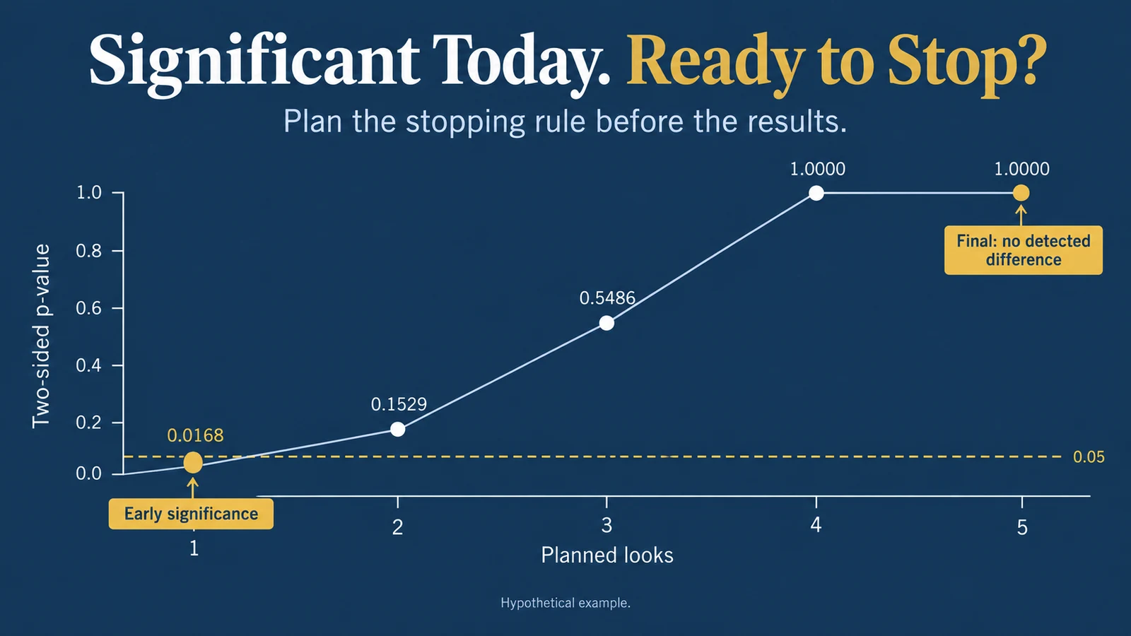
A product manager opens an experiment dashboard. The new checkout has a 15% conversion rate; control has 10%. The dashboard reports a two-sided p-value of 0.0168.
The team wants to stop the experiment and launch.
Yesterday, the result was not significant. Tomorrow, it might change again. The team has been checking after every block of new users, planning to stop whenever the ordinary p-value drops below 0.05.
That stopping rule changes the statistical question. A test calibrated for one planned analysis does not generally retain its nominal false-positive rate when the team repeatedly tests and selects the first favorable result.
This article examines that specific decision: when can an experiment stop for evidence of an effect? It assumes the assignment and measurement systems are functioning. Allocation integrity remains essential, but it is a separate diagnostic addressed in Your A/B Test Shows a 20% Lift. Can You Trust the Result?.
The Short Answer: The Stopping Rule Is Part of the Experiment
An experiment should specify how evidence will be evaluated before results influence the stopping decision.
Three possible approaches are:
- One planned final analysis at a fixed horizon.
- A finite set of interim analyses with an appropriate error-control plan.
- A validated sequential method designed to support monitoring over time.
These approaches offer different trade-offs. Merely refreshing a dashboard does not change observations. Using successive ordinary p-values to decide when to declare a winner changes the decision procedure.
The concern is not that an early result must be wrong. It is that the procedure can make false declarations more frequent than its label suggests.
What Does a 5% Significance Level Protect Against?
Under a correctly specified null model and a calibrated test, a significance level of 0.05 limits the probability of rejecting a true null hypothesis in repeated applications of that procedure.
It does not mean there is a 5% probability that a particular result is false. It does not mean the treatment has a 95% probability of working.
The procedure includes the sampling and decision rules. If the advertised test assumes a fixed analysis point, replacing that point with a data-dependent stopping time requires additional justification.
Johari, Pekelis, and Walsh develop always-valid inference specifically for online experiments with outcome-dependent monitoring. Their work explains why the inferential method and the stopping decision must be considered together. See their research preprint.
A Worked Example: Early Significance That Disappears
Consider a synthetic checkout experiment with stable user-level assignment. Each user has one binary conversion outcome, observed over the same completed outcome window.
For illustration, the experiment is reviewed after each additional 500 users per arm. These are five cumulative looks at the same experiment, not five independent experiments.
| Look | Users per Arm | Control Conversions | Treatment Conversions | Control Rate | Treatment Rate | Two-Sided p-value |
|---|---|---|---|---|---|---|
| 1 | 500 | 50 | 75 | 10.00% | 15.00% | 0.0168 |
| 2 | 1,000 | 100 | 120 | 10.00% | 12.00% | 0.1529 |
| 3 | 1,500 | 150 | 160 | 10.00% | 10.67% | 0.5486 |
| 4 | 2,000 | 200 | 200 | 10.00% | 10.00% | 1.0000 |
| 5 | 2,500 | 250 | 250 | 10.00% | 10.00% | 1.0000 |
All counts are hypothetical. They are not UAD Consulting client results. The sequence was constructed to make a timing issue visible; it is not evidence that real improvements usually disappear.
At Look 1, the absolute observed difference is five percentage points. The relative difference is (15% / 10%) - 1 = 50%.
At Look 2, the absolute difference is two percentage points and the relative difference is 20%. At the last look, the observed difference is zero.
Stopping at the first ordinary p-value below 0.05 would select Look 1. Continuing to the planned final look produces a different description of the accumulated data.
Neither pattern alone proves the underlying treatment effect. In particular, a final p-value of 1 does not establish equivalence or prove an exact zero effect. It reflects identical observed rates in this sample.
How the P-Values Were Calculated
The example uses the large-sample pooled two-proportion z-test under the null hypothesis of equal conversion probabilities.
Let c and t denote conversions, and n_c and n_t denote analyzed users in the two arms.
Pooled conversion estimate = (c + t) / (n_c + n_t).
Standard error under the null = sqrt[pooled × (1 - pooled) × (1/n_c + 1/n_t)].
z = (t/n_t - c/n_c) / standard error.
At the first look, the pooled rate is 125 / 1,000 = 0.125. The standard error is approximately 0.0209165. The observed difference, 0.05, gives z = 2.39046 and a two-sided normal-approximation p-value of approximately 0.0168274.
NIST documents this pooled two-proportion test. It requires suitable independent binary observations and adequate counts. Cluster-randomized experiments, repeated observations from the same user, and sparse outcomes need appropriate methods rather than automatic reuse of this calculation.
Reproduce the Five Looks in Python
This calculation uses only Python's standard library. It deliberately calculates ordinary fixed-look p-values; it does not convert them into sequentially valid evidence.
from math import erfc, sqrt

control = [50, 100, 150, 200, 250]
treatment = [75, 120, 160, 200, 250]

for look, (c, t) in enumerate(
    zip(control, treatment), start=1
):
    n = 500 * look
    pooled = (c + t) / (2 * n)
    standard_error = sqrt(
        pooled * (1 - pooled) * (2 / n)
    )
    z = (t / n - c / n) / standard_error
    p = erfc(abs(z) / sqrt(2))
    print(look, n, round(z, 5), round(p, 8))
The first two p-values are approximately 0.01682741 and 0.15291778. The distinction matters: observing a 20% relative lift at the second look does not itself establish adequate statistical evidence.
A launch decision also needs uncertainty around effect size, practical value, and business guardrails. A p-value alone cannot price implementation cost or customer risk.
A Simulation of 50,000 Experiments With No True Effect
One selected trajectory cannot quantify the long-run false-positive rate. To investigate the decision rule, simulate many experiments under an explicit null model.
Assume independent users, a constant 10% conversion probability in both arms, exactly 500 new users per arm per block, five blocks, and complete binary outcomes. Each simulated experiment has no true treatment effect.
Compare three two-sided rules:
- Test once after 2,500 users per arm, using p < 0.05.
- Test at all five looks and reject if any ordinary p-value is below 0.05.
- Preplan five looks and reject if any p-value is below 0.01.
The third rule applies a simple Bonferroni allocation: 0.05 / 5 = 0.01 per look.
Using the reproducible code below, the results are:
| Decision Rule | Null Experiments Rejected | Simulated False-Positive Percentage |
|---|---|---|
| One final analysis | 2,492 of 50,000 | 4.984% |
| Any of five unadjusted looks | 7,017 of 50,000 | 14.034% |
| Any of five Bonferroni-adjusted looks | 1,577 of 50,000 | 3.154% |
These are original simulation results under the stated assumptions, not measured platform performance or published benchmark rates.
The unadjusted procedure rejects substantially more often in this simulated setting. The exact inflation depends on the number and spacing of looks, their dependence, and the test and data-generating process.
The adjusted procedure is conservative here. This is not proof that 0.01 is the optimal threshold for all experiments.
Reproducible Simulation Code
This example uses NumPy, executed locally with NumPy 2.3.1. The seed and sampling order are explicit. Reproduction across other versions should verify the random-number implementation rather than assume identical bit-for-bit output.
from math import erfc, sqrt
import numpy as np

rng = np.random.default_rng(20261028)
trials, looks, block = 50000, 5, 500

control = np.cumsum(
    rng.binomial(block, 0.10, size=(trials, looks)),
    axis=1,
)
treatment = np.cumsum(
    rng.binomial(block, 0.10, size=(trials, looks)),
    axis=1,
)
n = block * np.arange(1, looks + 1)
pooled = (control + treatment) / (2 * n)
z = (treatment / n - control / n) / np.sqrt(
    pooled * (1 - pooled) * 2 / n
)
p = np.array([
    [erfc(abs(float(v)) / sqrt(2)) for v in row]
    for row in z
])

rules = {
    "final_only": p[:, -1] < 0.05,
    "unadjusted_any": (p < 0.05).any(axis=1),
    "bonferroni_any": (p < 0.01).any(axis=1),
}
for name, reject in rules.items():
    count = int(reject.sum())
    rate = count / trials
    mc_se = sqrt(rate * (1 - rate) / trials)
    print(name, count, round(100 * rate, 3), mc_se)
Monte Carlo standard errors are approximately 0.097, 0.155, and 0.078 percentage points, respectively. These quantify simulation variability, not uncertainty about a deployed checkout's business effect.
The conversion test itself uses a normal approximation. Consequently, finite-sample rejection rates need not equal the nominal level exactly. A production system should use methods appropriate to its own metric and randomization unit.
Why the Looks Are Not Independent
The second cumulative look includes users already present at the first look. Later estimates therefore share information.
It would be incorrect to describe the simulation as five independent tests or use 1 - (1 - 0.05)^5 as its exact false-positive probability. That expression applies to five independent rejection events with exactly 5% probability each.
The simulation preserves cumulative dependence by adding new binomial blocks and taking cumulative sums. That construction is central to the example.
Three Defensible Stopping Plans
Plan A: One Fixed Final Analysis
Define the sample size, minimum duration, outcome window, primary metric, and analysis method before viewing comparative results. Use an appropriate power calculation to choose the horizon; the illustrative 2,500 users per arm is not a sample-size recommendation.
Operational monitoring can continue. A crash or privacy incident may require stopping for safety regardless of statistical significance. Such a stop should be documented, and it does not make an ordinary early efficacy analysis valid.
A non-significant final result does not justify extending enrollment repeatedly until a favorable p-value appears. A redesign or new experiment may be appropriate, but its decision rule needs to be explicit.
Plan B: Preplanned Interim Analyses
Specify when interim analyses occur and how the error budget is distributed. A simple five-look Bonferroni plan uses 0.01 at each look, including the final one.
The union bound limits the chance of any false rejection to the sum of the individual error bounds; independence is not required. With valid per-look tests, five bounds of 0.01 imply an overall bound of 0.05. NIST explains the underlying Bonferroni inequality.
The guarantee is only as sound as the per-look tests. With approximate tests, finite-sample calibration must still be checked.
Bonferroni can sacrifice power. More efficient group-sequential designs can distribute error differently across planned looks. They require a coherent design, not an improvised adjustment after the observed path is known.
Plan C: Validated Continuous Monitoring
Always-valid p-values and time-uniform confidence sequences are designed for sequential use under their stated assumptions. A confidence sequence offers coverage across time, rather than the separate pointwise coverage of an ordinary interval at a single fixed look.
Howard, Ramdas, McAuliffe, and Sekhon provide a methodological foundation for time-uniform confidence sequences.
These tools do not remove measurement error, confounding from invalid exclusions, or experiment interference. Nor should an ordinary confidence interval be relabeled a confidence sequence. Confirm what the actual platform implementation guarantees for the metric being analyzed.
Audit the Decision Readouts in SQL
A stopping policy should leave an audit trail. The following portable SQL, compatible with PostgreSQL, compares recorded decision readouts with a stored plan.
Assume one planned row and at most one recorded decision readout per experiment and look number. Store timestamps in a consistent timezone and make the approved plan immutable or versioned before results are reviewed.
SELECT
    r.experiment_id,
    r.look_number,
    r.analysis_cutoff,
    p.planned_cutoff,
    p.alpha_per_look,
    CASE
        WHEN p.look_number IS NULL
            THEN 'unplanned_readout'
        WHEN r.analysis_cutoff <> p.planned_cutoff
            THEN 'cutoff_differs_from_plan'
        ELSE 'matches_plan'
    END AS audit_status
FROM experiment_readouts AS r
LEFT JOIN experiment_look_plan AS p
    ON r.experiment_id = p.experiment_id
   AND r.look_number = p.look_number
WHERE r.experiment_id = 'checkout_stopping_demo'
ORDER BY r.look_number;
The plan table contains experiment_id, look_number, planned_cutoff, and alpha_per_look. The readout table contains experiment_id, look_number, and analysis_cutoff. Keys, required fields, and null handling must be enforced; this query assumes non-null cutoff values.
A matching row does not certify statistical validity. This audit does not detect unrecorded informal peeking, establish outcome maturity, or validate the method used to calculate p-values. It makes one part of the analysis process inspectable.
Mature Outcomes Before Calling a Look Complete
A user assigned yesterday may still convert within a seven-day purchase window. Counting that user as a completed nonconverter can create a misleading readout.
Define the outcome window and when each user's outcome becomes eligible for analysis. Do not compare a fully matured control cohort with a partly observed treatment cohort.
Sequential inference does not automatically solve delayed outcomes. The procedure must support the observation and reveal process actually used. Align the data extraction rules with the statistical design and record a trustworthy analysis cutoff.
This is an implementation requirement for the stopping plan, not an invitation to choose whichever follow-up window produces the best result.
Do Not Turn an Early Estimate Into a Revenue Forecast
At the first look, the synthetic observed lift is 50%. Selecting that look because it is favorable also selects an unusually attractive estimate.
It would be inappropriate to multiply the 50% lift by annual traffic and call the result guaranteed revenue. Estimate precision, selection, customer mix, deployment conditions, and costs all matter.
Even a valid sequential rejection answers a hypothesis-testing question. It does not eliminate uncertainty around effect magnitude. Use effect estimates and intervals appropriate to the stopping design, then assess practical value and guardrails.
For the distinction between attribution and causal measurement, see Marketing Attribution vs. Incrementality. A credible experiment needs both a trustworthy population and an appropriate evidence-evaluation procedure.
A Decision Checklist Before Ending an Experiment
- Is the randomization unit stable, and have assignment and telemetry checks passed?
- Is the decision about safety, efficacy, futility, or an operational constraint?
- Was the stopping method chosen before comparative outcomes influenced the plan?
- Are all decision readouts included in the inferential procedure?
- Are outcomes mature and measured consistently?
- Are multiple variants, outcomes, and subgroup searches addressed separately?
- Do effect uncertainty and business guardrails support the proposed action?
Correcting for five looks does not automatically address dozens of searched metrics. Timing multiplicity and metric multiplicity can coexist. Document the full decision procedure instead of fixing one visible p-value.
The Result Is Not Just a Number on the Dashboard
The hypothetical checkout was significant at its first ordinary analysis and showed no observed difference at the final look. The accompanying null simulation showed why stopping at a favorable look changes the procedure's behavior across experiments.
This is not an argument against early decisions. It is an argument for designing them.
Before launch, establish whether the reported evidence remains valid under the stopping rule actually used. If the rule was improvised after viewing results, acknowledge that limitation rather than retroactively presenting the experiment as confirmatory.
A sound launch decision connects experiment integrity, valid inference, effect uncertainty, and business consequences. The point at which the team chooses to stop is part of that evidence.
References and Methodological Notes
Johari, R., Pekelis, L., and Walsh, D. J. Always Valid Inference: Bringing Sequential Analysis to A/B Testing. Research preprint, first submitted 2015, revised 2019. arXiv:1512.04922. https://arxiv.org/abs/1512.04922
Howard, S. R., Ramdas, A., McAuliffe, J., and Sekhon, J. (2021). Time-uniform, nonparametric, nonasymptotic confidence sequences. The Annals of Statistics, 49(2), 1055–1080. DOI: 10.1214/20-AOS1991. Author manuscript and journal details: https://arxiv.org/abs/1810.08240
NIST/SEMATECH Engineering Statistics Handbook. How can we determine whether two processes produce the same proportion of defectives? Section 7.3.3. https://www.itl.nist.gov/div898/handbook/prc/section3/prc33.htm
NIST/SEMATECH Engineering Statistics Handbook. Bonferroni's method. Section 7.4.7.3. https://www.itl.nist.gov/div898/handbook/prc/section4/prc473.htm
Methodological Note
All counts, trajectories, SQL fixtures, and simulation results are synthetic educational examples. They are not actual UAD Consulting analytics, client data, or measured commercial effects. The worked trajectory is deliberately constructed. The null simulation uses independent Bernoulli outcomes with constant probabilities and five cumulative looks; it does not model every source of real experiment heterogeneity. The z-tests are normal approximations. The Bonferroni bound relies on valid individual tests. The SQL is an audit example, not an experimentation engine. No example establishes a causal benefit or a universal stopping threshold.
Make Experiment Results Decision-Ready
Reliable experiments connect trustworthy measurement, appropriate statistical methods, and clear business decisions.
UAD Consulting helps organizations examine experimentation design, marketing measurement, and analytical workflows before translating results into operational decisions.
Explore our Marketing & Digital Analytics services or get in touch to discuss your experimentation and measurement challenges.
Explore ServicesGet in Touch