A retailer uses a forecasting model to estimate weekly product demand.
Its analytics dashboard reports a forecast error of 30%.
Management wants to know whether the model is good enough to support purchasing decisions.
But 30% of what?
Does the number mean the model is wrong by 30 units for every 100 sold?
Does it mean demand was underestimated?
Does it mean the business should hold more inventory?
And would a model with a lower error score necessarily produce better inventory decisions?
The answers depend on how forecast accuracy is measured and what the business is trying to optimize.
Forecasting is not simply an exercise in predicting the next number.
For a retailer, distributor, hospital supply department, or manufacturing business, forecasts influence purchasing, staffing, replenishment, and capacity decisions.
A forecast can perform well statistically while creating expensive operational consequences.
The useful question is therefore not only:
"Which model has the lowest forecast error?"
It is also:
"Which forecast supports the best decision under the costs and constraints our business actually faces?"
The Short Answer: Forecast Accuracy and Decision Quality Are Different
Forecast accuracy measures how closely predictions match observed outcomes.
Decision quality concerns whether actions based on those predictions produce desirable results.
The two are related, but they are not interchangeable.
A forecasting model may have a low average error while consistently underestimating demand for high-priority products.
Another model may have a slightly higher average error but produce fewer costly shortages.
The preferred model depends on the decision.
For inventory planning, relevant considerations can include:
- Forecast error magnitude
- Direction of forecast bias
- Product demand frequency
- Lead times
- Holding costs
- Shortage costs
- Service-level requirements
- Replenishment constraints
- Demand uncertainty
No single forecast accuracy metric captures all these dimensions.
This distinction connects to a broader principle in predictive analytics: model performance should be evaluated in relation to the decision the model supports.
For a related discussion, see UAD Consulting's article:
From Predictive Analytics to Decision-Making
What Is MAPE?
Mean Absolute Percentage Error, or MAPE, is a widely used forecasting metric.
It measures the average absolute percentage difference between actual values and forecasts.
For n observations:
For example, suppose actual demand is 100 units and the forecast is 90 units.
Absolute percentage error:
|100 - 90| / 100 × 100
= 10%.
For one observation, the absolute percentage error is 10%.
Across multiple observations, MAPE averages these percentages.
This makes MAPE relatively easy to explain.
However, the metric has important limitations.
Problem 1: Zero Demand
Suppose a product has zero sales in a particular week.
Actual demand = 0.
Forecast demand = 3.
The absolute percentage error would require:
|0 - 3| / 0.
That expression is undefined.
Products with intermittent demand frequently have zero-demand periods.
MAPE therefore cannot be calculated conventionally across those observations.
Simply deleting zero-demand weeks changes the evaluation population and may make the model appear more accurate than it is.
Problem 2: Small Actual Values
Suppose actual demand is one unit and the forecast is four units.
Absolute percentage error:
|1 - 4| / 1 × 100
= 300%.
A three-unit error produces a 300% percentage error.
Meanwhile, an error of three units when actual demand is 100 produces only 3%.
This behavior may be appropriate for some applications.
But it can make MAPE difficult to interpret when demand varies substantially across products or periods.
Problem 3: Business Costs Are Not Represented
MAPE treats overforecasting and underforecasting symmetrically in absolute-error terms.
However, businesses may face very different consequences.
Underforecasting can produce shortages.
Overforecasting can produce excess inventory.
The costs are not necessarily equal.
Hyndman and Koehler (2006) examined limitations of commonly used forecasting accuracy measures and proposed mean absolute scaled error as an alternative.
Their research provides an important methodological foundation for evaluating forecasting models across different types of time series.
What Is WAPE?
Weighted Absolute Percentage Error, or WAPE, is commonly calculated as:
Multiply by 100 to express the result as a percentage.
Unlike MAPE, WAPE calculates the ratio using aggregate absolute error and aggregate actual volume.
Consider three weeks:
| Week | Actual Demand | Forecast | Absolute Error |
|---|---|---|---|
| 1 | 100 | 90 | 10 |
| 2 | 200 | 180 | 20 |
| 3 | 300 | 270 | 30 |
| Total | 600 | 540 | 60 |
WAPE:
60 / 600 × 100
= 10%.
WAPE is often useful when evaluating forecasts across products or periods with different volumes.
A ten-unit error on a high-volume product contributes the same absolute error as a ten-unit error on a low-volume product.
But the aggregate denominator is driven by total observed volume.
This makes the metric relatively sensitive to errors in high-volume parts of the business.
However, WAPE is not a universal solution.
WAPE Can Still Be Undefined
If every actual observation in the evaluation period is zero:
SUM(|Actual|) = 0.
The denominator is zero.
WAPE is undefined.
This can occur when evaluating slow-moving inventory over a short period.
WAPE Can Change With the Evaluation Period
Rob Hyndman has highlighted another limitation.
Because WAPE uses actual values from the evaluation period in its denominator, changes in the level or structure of demand can affect the score.
For example, when demand grows over time, the denominator may increase even if the underlying forecasting errors do not improve proportionally.
A falling WAPE does not automatically demonstrate improving forecasting capability.
This is particularly important when comparing performance across periods with different demand patterns.
Source:
Rob J. Hyndman. WAPE: Weighted Absolute Percentage Error.
https://robjhyndman.com/hyndsight/wape.html
What Is MASE?
Mean Absolute Scaled Error, or MASE, evaluates forecast errors relative to a benchmark scale calculated from historical training data.
For a nonseasonal time series, a common denominator is the average absolute one-step change in the training observations.
Here:
Test MAE is the mean absolute forecast error on the evaluation period.
Training Naive MAE is the mean absolute error associated with the one-step naive benchmark calculated from the training series.
For a nonseasonal naive forecast, the next value is predicted using the previous observed value.
MASE is useful because it places errors on a scale related to historical variation.
It can help compare forecasting performance across series with different measurement scales.
However, MASE also requires care.
The benchmark denominator must be defined consistently.
Seasonal series may require a seasonal naive benchmark.
If the historical training series is constant, the usual naive-error denominator is zero and conventional MASE becomes undefined.
A low MASE is not a guarantee of good inventory performance.
It remains a statistical error metric.
Hyndman and Koehler (2006) provide the methodological foundation for MASE.
Reference:
Hyndman RJ, Koehler AB.
Another look at measures of forecast accuracy.
International Journal of Forecasting. 2006;22(4):679-688.
https://doi.org/10.1016/j.ijforecast.2006.03.001
A Worked Example: Two Models With Identical Forecast Accuracy
Consider a hypothetical retailer selling a product with intermittent weekly demand.
The company evaluates two forecasting models over six weeks.
The observed demand is:
0, 0, 0, 8, 0, 12 units.
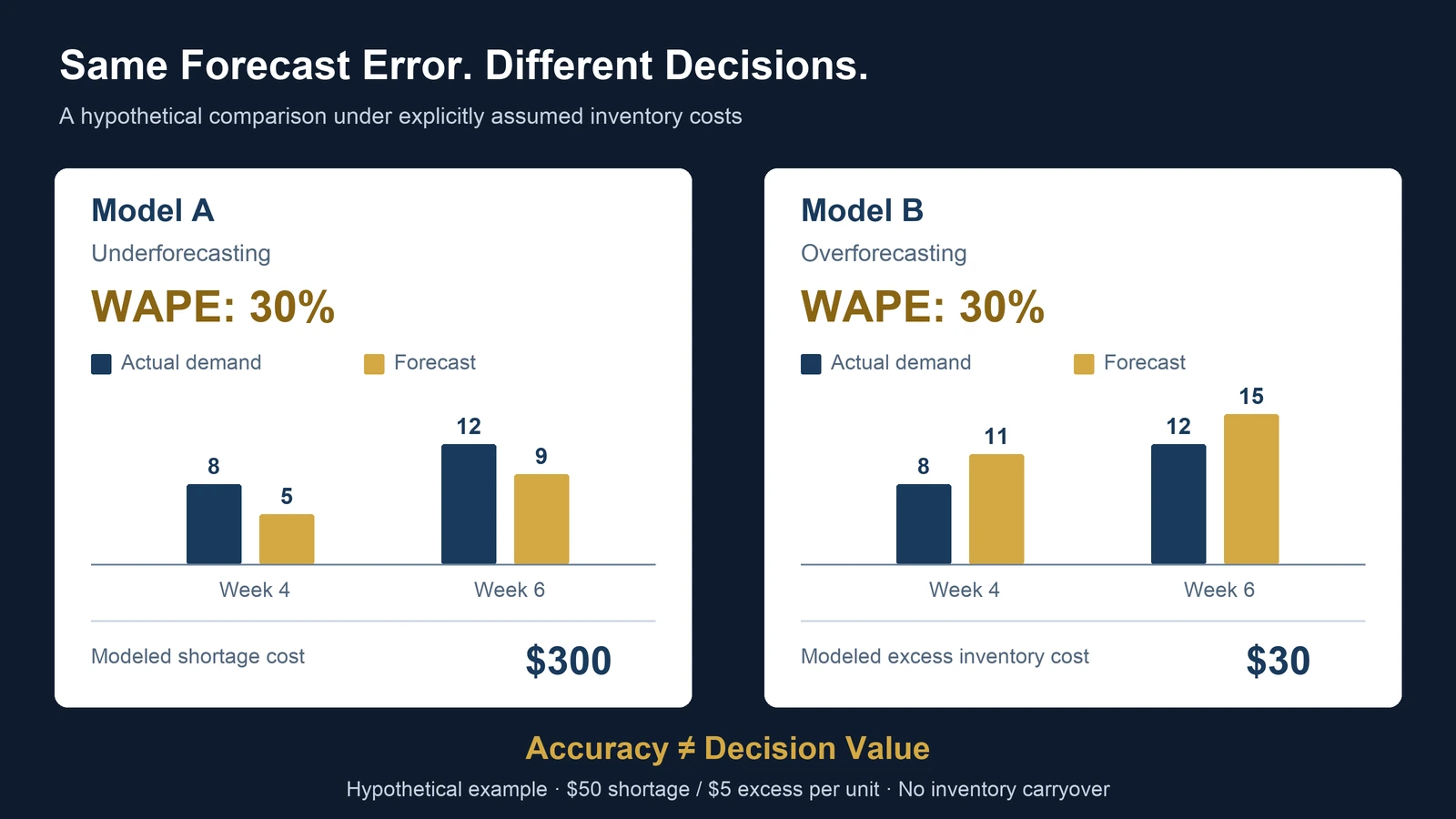
Model A tends to underestimate demand.
Model B tends to overestimate demand.
Assume the following forecasts.
| Week | Actual Demand | Model A | Model B |
|---|---|---|---|
| 1 | 0 | 0 | 0 |
| 2 | 0 | 0 | 0 |
| 3 | 0 | 0 | 0 |
| 4 | 8 | 5 | 11 |
| 5 | 0 | 0 | 0 |
| 6 | 12 | 9 | 15 |
| Total | 20 | 14 | 26 |
All values are hypothetical.
They are not actual UAD Consulting client results.
The example is deliberately simple to isolate the consequences of forecast direction.
Step 1: Calculate Model A's Absolute Error
For Model A:
Week 1: |0 - 0| = 0
Week 2: |0 - 0| = 0
Week 3: |0 - 0| = 0
Week 4: |8 - 5| = 3
Week 5: |0 - 0| = 0
Week 6: |12 - 9| = 3
Total absolute error:
0 + 0 + 0 + 3 + 0 + 3 = 6 units.
Step 2: Calculate Model B's Absolute Error
For Model B:
Week 1: |0 - 0| = 0
Week 2: |0 - 0| = 0
Week 3: |0 - 0| = 0
Week 4: |8 - 11| = 3
Week 5: |0 - 0| = 0
Week 6: |12 - 15| = 3
Total absolute error:
0 + 0 + 0 + 3 + 0 + 3 = 6 units.
Both models produce the same total absolute error.
Step 3: Calculate WAPE
Total actual demand:
20 units.
Model A:
= 30%.
Model B:
= 30%.
The two models have identical WAPE.
Step 4: Calculate MAE
Mean Absolute Error:
MAE = Total Absolute Error / Number of Observations
Model A:
6 / 6 = 1 unit per week.
Model B:
6 / 6 = 1 unit per week.
Again, the models are identical according to the metric.
Step 5: Calculate MASE
Suppose the historical training observations were:
0, 4, 0, 0, 8, 0, 0.
The absolute consecutive changes are:
4, 4, 0, 8, 8, 0.
Total absolute consecutive change:
24.
There are six consecutive differences.
Training naive MAE:
24 / 6 = 4.
The test MAE for each model is one unit.
Therefore:
Model A MASE = 1 / 4 = 0.25.
Model B MASE = 1 / 4 = 0.25.
The two models have identical MASE under this shared training benchmark.
The result is a useful reminder.
Changing the accuracy metric does not necessarily resolve the business decision.
Both models have the same MAE, WAPE, and MASE in this example.
Yet their forecasting errors point in opposite directions.
The Missing Information: Forecast Bias
Forecast bias concerns the direction of forecasting errors.
Define signed forecast error as:
Forecast - Actual.
Under this convention:
Positive values indicate overforecasting.
Negative values indicate underforecasting.
For Model A:
Total forecast demand = 14.
Total actual demand = 20.
Signed error:
14 - 20 = -6.
Model A underforecasts by six units across the evaluation period.
For Model B:
Total forecast demand = 26.
Total actual demand = 20.
Signed error:
26 - 20 = +6.
Model B overforecasts by six units.
The average signed errors are:
Model A: -6 / 6 = -1 unit per week.
Model B: +6 / 6 = +1 unit per week.
The models have equal absolute error but opposite signed bias over the six observed weeks.
This is a descriptive result for the example.
It does not establish that either model will remain biased in future periods.
Forecast bias should be monitored across repeated evaluation windows and relevant product groups.
The Business Decision: Which Model Is Actually Better?
Now introduce inventory economics.
Assume the retailer orders exactly the quantity predicted for each week.
For this simplified illustration:
- There is no beginning inventory.
- Orders arrive immediately before the week's demand.
- Unused inventory does not carry into another week.
- Each unfulfilled unit incurs a $50 shortage penalty.
- Each excess unit incurs a $5 overage cost.
- No other costs or constraints are included.
These assumptions intentionally simplify real inventory operations.
They are not a recommended production replenishment policy.
Model A: Underforecasting
Model A underforecasts by three units in Week 4 and three units in Week 6.
Total shortage:
6 units.
Shortage cost:
6 × $50 = $300.
There is no excess inventory under the simplified example.
Total modeled cost:
$300.
Model B: Overforecasting
Model B overforecasts by three units in Week 4 and three units in Week 6.
Total excess inventory:
6 units.
Overage cost:
6 × $5 = $30.
There are no shortages under the simplified example.
Total modeled cost:
$30.
Compare the Results
| Metric | Model A | Model B |
|---|---|---|
| MAE | 1.00 | 1.00 |
| WAPE | 30% | 30% |
| MASE | 0.25 | 0.25 |
| Total signed error | -6 | +6 |
| Shortage units | 6 | 0 |
| Excess units | 0 | 6 |
| Modeled inventory cost | $300 | $30 |
Both models have identical accuracy scores.
Yet under the stated assumptions, Model B produces $270 less inventory cost.
Cost difference:
$300 - $30 = $270.
This is a 90% reduction relative to Model A's modeled cost.
The result is not evidence that overforecasting is universally preferable.
It demonstrates that the preferred forecast depends on the economic consequences of errors.
If excess inventory were very expensive, the comparison could change.
If the product were perishable, the overage penalty might be much higher.
If shortages caused minimal business disruption, the shortage penalty might be lower.
If inventory carried forward, the simple weekly cost calculation would no longer apply.
The assumptions determine the result.
Why Forecast Accuracy Alone Cannot Determine Inventory Policy
Inventory planning involves a decision under uncertainty.
A forecast estimates future demand.
A replenishment policy determines how much to order.
Those are related but separate decisions.
A business may use the same demand forecast with different inventory policies depending on:
- Target service level
- Supplier lead time
- Demand variability
- Inventory already on hand
- Storage capacity
- Product shelf life
- Shortage consequences
- Holding costs
- Ordering costs
For example, a business with expensive shortages may deliberately order above its central demand forecast.
That does not necessarily mean the forecasting model is biased.
It may mean the replenishment policy incorporates a rational safety margin.
This distinction matters.
Forecast bias describes systematic directional error in the prediction.
Safety stock is a deliberate inventory decision intended to manage uncertainty.
They should not be confused.
A decision-aware forecasting evaluation should therefore examine the forecast and the replenishment policy separately.
What If the Business Has Hundreds of Products?
The problem becomes more complicated when evaluating many stock-keeping units, or SKUs.
A company may have:
- High-volume products
- Low-volume products
- Seasonal products
- Intermittent-demand products
- High-margin products
- Products with long supplier lead times
- Products with substantial shortage penalties
A single portfolio-wide WAPE can conceal important differences.
Because WAPE uses aggregate absolute volume, high-volume products can dominate the result.
An improvement in forecasts for one large product category may reduce portfolio WAPE while performance deteriorates for critical low-volume products.
That does not make WAPE useless.
It means the metric should be interpreted according to the decision.
A practical forecast evaluation dashboard may report:
| Measurement | Primary Question |
|---|---|
| MAE | How many units are forecasts wrong by on average? |
| WAPE | How large is aggregate absolute error relative to observed volume? |
| MASE | How does error compare with a historical naive benchmark scale? |
| Signed bias | Does the forecast systematically overestimate or underestimate? |
| Shortage units | How much demand would the specified policy fail to fulfill? |
| Excess inventory | How much inventory would remain under the specified policy? |
| Modeled inventory cost | What are the economic consequences under stated assumptions? |
| Service-level attainment | Does the policy meet the operational service target? |
The appropriate combination depends on the business.
For example, a hospital supply department may place greater emphasis on availability for critical items.
A retailer selling highly perishable products may emphasize the cost of unsold inventory.
A distributor may need to balance both.
These decisions cannot be resolved through forecast accuracy alone.
Why Forecast Validation Must Respect Time
Forecasting models should be evaluated using information that would have been available when each forecast was made.
Randomly splitting historical time-series observations into training and testing datasets can allow future information to influence predictions of earlier periods.
That can produce misleading performance estimates.
A more appropriate approach is rolling-origin evaluation.
The analyst repeatedly:
- Selects a historical forecast origin.
- Trains using information available up to that point.
- Produces forecasts for the required future horizon.
- Compares those forecasts with subsequently observed outcomes.
- Advances the forecast origin.
- Repeats the evaluation.
This produces a collection of historical out-of-sample forecasts.
The evaluation should reflect the actual business forecasting horizon.
A business ordering inventory six weeks ahead should not select its forecasting model solely using one-week-ahead accuracy.
The relevant forecast horizon should match the replenishment decision.
Hyndman and Athanasopoulos explain rolling-origin evaluation in Forecasting: Principles and Practice.
Reference:
https://otexts.com/fpp3/tscv.html
What Should a Forecast Evaluation Report Include?
A useful report should make the following information explicit.
Forecast Definition
What is being predicted?
Examples include:
Weekly product demand.
Daily customer arrivals.
Monthly sales.
Quarterly service utilization.
Forecast Horizon
How far ahead is the prediction made?
One day?
One week?
Six weeks?
Three months?
Evaluation Population
Which products, locations, customers, or periods are included?
Customer-based forecasts also require consistent customer identities.
Were zero-demand observations retained?
Were discontinued products excluded?
Were only successful forecasts selected?
Statistical Accuracy
Which error metrics are reported?
Are their denominators defined?
Are undefined values handled transparently?
Forecast Bias
Does the model systematically overforecast or underforecast?
Does the direction vary across product groups?
Operational Consequences
How do forecast errors affect inventory, staffing, capacity, or service outcomes?
Economic Assumptions
What costs are associated with different decisions?
How sensitive are the conclusions to those assumptions?
Uncertainty
How stable are the results across historical evaluation windows?
Are differences large enough to matter operationally?
This structure is more useful than a dashboard displaying one forecast accuracy percentage without context.
For related guidance on building decision-focused metrics, see:
A KPI Framework for Business Analytics
A Practical Framework for Selecting Forecasting Models
A business can evaluate forecasting models through five stages.
Stage 1: Define the Decision
Start with the operational question.
How much inventory should be ordered?
How many employees should be scheduled?
How much capacity is required?
The decision determines the relevant forecast horizon and error consequences.
Stage 2: Establish Simple Benchmarks
Compare candidate models with appropriate baseline methods.
For example, a seasonal naive forecast may be a useful benchmark for seasonal demand.
A more complex model should demonstrate value beyond complexity alone.
Stage 3: Evaluate Statistical Accuracy
Calculate appropriate metrics such as MAE, WAPE, or MASE.
Document zero-demand handling and denominator limitations.
Compare performance using historical out-of-sample forecasts.
Stage 4: Evaluate Decision Consequences
Translate forecasts into decisions using a defined operational policy.
Estimate relevant costs and service outcomes.
Do not assume that lower statistical error automatically produces lower business cost.
Stage 5: Test Sensitivity
Vary important assumptions.
For inventory, these might include:
Shortage cost.
Holding cost.
Lead time.
Demand variability.
Service-level target.
If the preferred model changes under plausible assumptions, the recommendation should acknowledge that uncertainty.
The final selection should reflect both forecasting performance and the decision environment.
Can Better Forecast Accuracy Cause Better Business Performance?
Improved forecast accuracy may support better decisions.
However, observing that forecast accuracy and business performance improve together does not establish causality.
Inventory costs may change because of:
- Supplier changes
- Pricing decisions
- Demand shifts
- Replenishment policy changes
- Product assortment changes
- Operational improvements
- Seasonality
A model comparison using the same historical demand data and the same explicitly specified inventory policy can estimate differences in modeled outcomes.
But that is a model-based comparison.
It is not necessarily a causal estimate of the effect of deploying one forecasting system in a real business.
A credible operational evaluation should account for implementation differences, policy changes, and external factors.
When appropriate, a controlled rollout or carefully designed experiment may provide stronger evidence of real-world impact.
The distinction is important.
Forecast evaluation measures predictive performance.
Decision modeling estimates consequences under assumptions.
Causal evaluation attempts to estimate what changed because an intervention occurred.
These are complementary analytical activities, not interchangeable ones.
The Bottom Line: The Best Forecast Is Not Always the One With the Lowest Error
MAPE, WAPE, and MASE can provide useful information about forecasting performance.
But each metric has limitations.
MAPE is problematic when actual demand is zero.
WAPE can be undefined when total actual demand is zero and can be difficult to compare across changing demand patterns.
MASE provides a useful historical benchmark scale but still does not represent business costs directly.
Our hypothetical example demonstrates the central issue.
Two models produced identical MAE, WAPE, and MASE.
Yet one generated $300 in modeled shortage costs while the other generated $30 in modeled excess inventory costs.
The difference came from the direction of the errors and the economic assumptions—not the magnitude of statistical error.
A strong forecasting workflow should therefore connect:
Demand data → Forecast → Accuracy evaluation → Operational policy → Business outcome.
The objective is not simply to predict the future more accurately.
It is to make better decisions with the uncertainty that remains.
References and Methodological Notes
Hyndman, R. J., & Koehler, A. B. (2006).
Another look at measures of forecast accuracy.
International Journal of Forecasting, 22(4), 679–688.
Hyndman, R. J.
WAPE: Weighted Absolute Percentage Error.
Hyndman, R. J., & Athanasopoulos, G. (2021).
Forecasting: Principles and Practice, 3rd edition.
OTexts.
Hyndman, R. J., & Athanasopoulos, G.
Time Series Cross-Validation.
Forecasting: Principles and Practice.
Hyndman, R. J. (2026).
Rolling Scaled Forecast Accuracy.
Methodological Note
All numerical examples are original hypothetical illustrations.
They do not represent actual UAD Consulting client data or observed commercial results.
The worked example uses simplified inventory assumptions to isolate the economic consequences of forecast direction.
Real inventory systems involve additional considerations such as lead times, beginning inventory, replenishment frequency, order quantities, service levels, and uncertainty.
The example should not be used directly to determine inventory purchasing decisions without a context-specific evaluation.
Turn Better Forecasts Into Better Decisions
Forecast accuracy is only part of effective planning.
UAD Consulting approaches predictive analytics, forecasting, and scenario modeling by connecting statistical evidence with operational decisions and business trade-offs.
Explore our Predictive Analytics & Modeling services or get in touch to discuss your forecasting challenge.
Explore ServicesGet in Touch