A retail business is considering opening a second location.
The proposed property looks promising.
It is close to residential neighborhoods, has good road access, and appears to serve a substantial customer market.
An initial market analysis estimates that the new location could generate approximately $156,000 in annual sales.
Management is encouraged.
The company already operates a profitable store, and a second location appears to offer a straightforward opportunity for growth.
But one important question remains:
Where will those sales come from?
Some customers may currently shop with competitors.
Others may already shop at the company's existing location.
If a customer simply switches from the original store to the new store, the company records revenue at the new location without necessarily increasing total company revenue.
This is retail cannibalization.
It is a critical consideration in store expansion, restaurant development, branch planning, and other location-based business decisions.
A useful location analysis should therefore distinguish three quantities:
- Gross revenue expected at the proposed site.
- Revenue displaced from existing company locations.
- Incremental revenue gained by the business as a whole.
This article develops a hypothetical example using the Huff model, a probabilistic spatial interaction framework that incorporates location attractiveness and travel impedance.
The objective is not to predict the performance of a particular real-world store.
It is to demonstrate how location analytics can improve the structure of an expansion decision.
The Short Answer: New Store Sales Are Not Necessarily New Company Sales
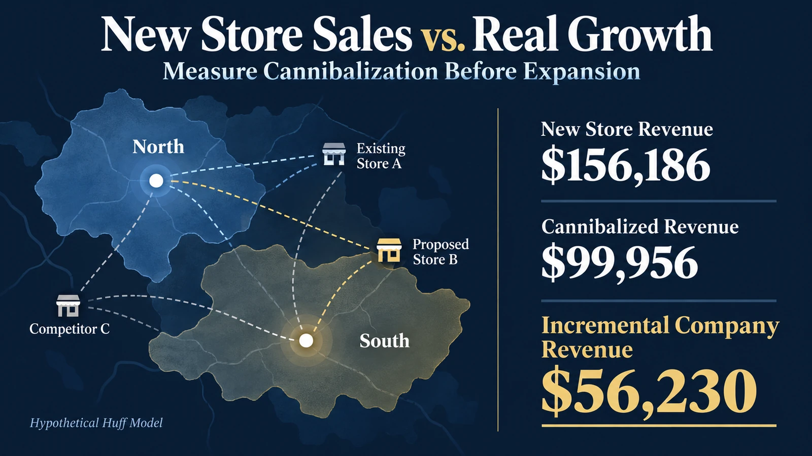
Suppose a proposed location is expected to generate:
$156,186 in annual revenue.
A business might initially treat this as an additional $156,186 in sales.
But imagine the location draws approximately $99,956 away from an existing company store.
The incremental company revenue becomes:
$156,186 - $99,956
= $56,230.
Approximately 64% of the proposed location's revenue represents sales displaced from the existing location.
Only 36% represents additional company revenue under the model.
This does not automatically mean the new store is a bad investment.
It may improve customer access, reduce congestion, serve strategic objectives, or create future growth opportunities.
But it changes the financial question.
Instead of asking:
"How much will the new store sell?"
Management should ask:
"How much additional economic value will the new store create for the company?"
What Is Retail Cannibalization?
Retail cannibalization occurs when a new location captures business that would otherwise have gone to an existing location owned by the same company.
Consider a customer who currently travels 15 minutes to an established store.
The company opens another location only eight minutes away.
The customer begins shopping at the new location.
The new store reports a sale.
The original store loses a sale.
From the company's perspective, the transaction may simply have moved between locations.
This is different from capturing a customer who previously purchased from a competitor.
That second transaction may increase company revenue.
The distinction is important because location-level reporting can create misleading impressions.
A new branch may appear successful while the overall business grows only modestly.
Cannibalization is not necessarily undesirable.
A company may deliberately accept some cannibalization to improve convenience, protect market share, increase service capacity, or prevent competitors from entering an area.
But the tradeoff should be quantified rather than ignored.
Why Distance Alone Is Not Enough
A simple site-selection analysis might assume that customers always visit the nearest store.
That assumption is easy to understand.
It is also frequently too restrictive.
Customers may consider:
- Travel time.
- Store size.
- Product assortment.
- Brand familiarity.
- Service quality.
- Parking availability.
- Operating hours.
- Price.
- Convenience.
- Competing alternatives.
A larger or more attractive store may draw customers from farther away.
A nearby store may attract relatively little demand if it offers a weaker experience.
Location models therefore often combine distance or travel time with some measure of attractiveness.
The Huff model is one established way to represent this relationship.
What Is the Huff Model?
The Huff model estimates the probability that demand originating from a geographic area is allocated to a particular retail location.
The probability depends on the location's attractiveness relative to competing alternatives and the travel impedance between the demand area and each location.
A simplified formulation is:
P_ij = [A_j / T_ij^beta]
       /
       SUM_k [A_k / T_ik^beta]
Where:
- P_ij is the modeled probability that demand from area i selects location j.
- A_j is the attractiveness score of location j.
- T_ij is the travel time or another positive impedance measure between demand area i and location j.
- beta is the distance-decay parameter.
The denominator includes all modeled competing locations.
A larger attractiveness score increases the location's relative weight.
A longer travel time reduces its relative weight when beta is positive.
The model produces probabilities that sum to one across the included alternatives for each demand area.
This is a conditional model of choice among the specified locations.
It is not automatically a model of whether a customer will shop in the category at all.
The probabilities are model outputs conditional on the demand areas, choice set, attractiveness values, and travel impedances supplied to the analysis. They are not measured visit frequencies, observed customer choices, or evidence that opening a site causes a particular customer to switch stores.
Esri's ArcGIS Business Analyst documentation describes the Huff model as a method for estimating spatial sales potential using distance and attractiveness.
The model is useful for scenario analysis, but its parameters require validation against the relevant market.
A Worked Example: One Existing Store, One Competitor, and One Proposed Location
Consider a hypothetical retail company.
It currently operates Store A.
A competitor operates Store C.
The company is considering opening Store B.
The relevant market is divided into two simplified demand areas:
North.
South.
The example assumes that annual category spending across these areas totals:
$300,000.
North contributes:
$200,000.
South contributes:
$100,000.
The example assumes a fixed amount of spending allocated among the modeled stores.
It does not include online purchases, an outside option, or changes in total category demand.
All inputs are synthetic.
They are not based on actual customers, locations, or sales records.
Define Store Attractiveness and Travel Time
Assume the following attractiveness scores.
Store A:
100.
Store C:
80.
Proposed Store B:
120.
These are hypothetical relative scores.
They are not measured customer preferences.
In a real application, attractiveness might be modeled using store size, product assortment, accessibility, service features, or other variables supported by evidence.
Now assume the following travel times.
| Location | North | South | Attractiveness |
|---|---|---|---|
| Existing Store A | 10 min | 15 min | 100 |
| Competitor C | 15 min | 10 min | 80 |
| Proposed Store B | 8 min | 12 min | 120 |
For the worked example, use:
beta = 2.
The resulting location weight is:
Weight = Attractiveness / Travel Time².
The exponent is an illustrative assumption.
It is not an empirically calibrated estimate for this market.
Step 1: Estimate the Market Before Opening Store B
Initially, customers choose between:
Store A.
Competitor C.
For the North area:
Store A weight:
100 / 10² = 1.0000.
Competitor C weight:
80 / 15² = 0.3556.
Total weight:
1.3556.
Store A's modeled share:
1.0000 / 1.3556
= approximately 73.77%.
Competitor C's modeled share:
Approximately 26.23%.
For the South area:
Store A weight:
100 / 15² = 0.4444.
Competitor C weight:
80 / 10² = 0.8000.
Total weight:
1.2444.
Store A's modeled share:
Approximately 35.71%.
Competitor C's modeled share:
Approximately 64.29%.
The baseline allocation is:
| Demand Area | Store A Share | Competitor C Share |
|---|---|---|
| North | 73.77% | 26.23% |
| South | 35.71% | 64.29% |
Now apply these shares to the annual demand assumptions.
North revenue allocated to Store A:
$200,000 × 73.7705%
= approximately $147,541.
South revenue allocated to Store A:
$100,000 × 35.7143%
= approximately $35,714.
Total baseline revenue allocated to Store A:
Approximately $183,255.
The remaining modeled market revenue goes to Competitor C:
Approximately $116,745.
These are model allocations, not measured sales.
Step 2: Add the Proposed Store
Now include Store B in the choice set.
For North:
Store B weight:
120 / 8² = 1.8750.
The combined weights become:
Store A: 1.0000.
Store B: 1.8750.
Competitor C: 0.3556.
Total:
3.2306.
The resulting modeled shares are approximately:
Store A: 30.95%.
Store B: 58.04%.
Competitor C: 11.01%.
For South:
Store B weight:
120 / 12² = 0.8333.
The combined weights become:
Store A: 0.4444.
Store B: 0.8333.
Competitor C: 0.8000.
Total:
2.0778.
The modeled shares become approximately:
Store A: 21.39%.
Store B: 40.11%.
Competitor C: 38.50%.
The updated allocation is:
| Demand Area | Store A | New Store B | Competitor C |
|---|---|---|---|
| North | 30.95% | 58.04% | 11.01% |
| South | 21.39% | 40.11% | 38.50% |
The new location attracts substantial demand.
But the model does not yet tell us how much of that demand is incremental to the company.
For that, we need to compare company-wide revenue before and after the proposed opening.
Step 3: Calculate New Store Revenue
Store B's modeled North revenue is:
$200,000 × 58.0396%
= approximately $116,079.
Its modeled South revenue is:
$100,000 × 40.1070%
= approximately $40,107.
Total projected revenue for Store B:
$116,079 + $40,107
= approximately $156,186.
This is the number that might appear in a conventional site feasibility report.
On its own, it looks encouraging.
But it is not the same as incremental company revenue.
Step 4: Calculate Cannibalization
Before opening Store B, the existing company location had modeled annual revenue of:
$183,255.
After adding Store B, Store A's modeled revenue becomes:
$83,299.
The reduction is:
$183,255 - $83,299
= approximately $99,956.
This is the modeled revenue displaced from the company's existing location.
Now compare that loss with the new store's revenue.
Cannibalization ratio:
$99,956 / $156,186
= approximately 64.0%.
Under the model, approximately 64% of Store B's projected revenue comes from sales that would otherwise have been allocated to Store A.
This is not an empirical cannibalization estimate.
It is a scenario result conditional on the model inputs and assumptions.
Step 5: Calculate Incremental Company Revenue
The business owns Stores A and B.
Therefore, company-wide revenue after opening the proposed location is:
Store A revenue + Store B revenue.
Approximately:
$83,299 + $156,186
= $239,485.
Before opening Store B, the company had:
$183,255.
The modeled incremental company revenue is:
$239,485 - $183,255
= approximately $56,230.
We can also calculate the same result directly:
New Store Revenue - Cannibalized Existing Revenue.
$156,186 - $99,956
= approximately $56,230.
The two methods agree, subject to rounding.
The result is summarized below.
| Measure | Annual Modeled Revenue |
|---|---|
| Company before expansion | $183,255 |
| Existing Store A after expansion | $83,299 |
| New Store B | $156,186 |
| Company after expansion | $239,485 |
| Existing-store cannibalization | $99,956 |
| Incremental company revenue | $56,230 |
The difference between $156,186 and $56,230 is central to the expansion decision.
The new location may generate substantial revenue without producing an equally large increase in company-wide revenue.
Step 6: Translate Revenue Into Economic Value
Revenue alone does not establish whether expansion is financially attractive.
Suppose the company uses a hypothetical incremental contribution margin of:
35%.
This margin should represent revenue remaining after the variable costs relevant to the expansion decision.
The modeled additional annual contribution before new location fixed costs is:
$56,230 × 35%
= approximately $19,681.
Now assume the new location introduces:
$30,000 in incremental annual fixed operating costs.
The modeled annual incremental operating contribution becomes:
$19,681 - $30,000
= approximately -$10,319.
Under these assumptions, opening the second location reduces annual operating contribution.
The new store has substantial projected gross sales.
But the incremental company-wide economics are negative.
This example excludes initial capital investment, financing, taxes, depreciation, working capital, and other potential consequences.
It is a simplified operating comparison, not a complete investment valuation.
What Is the Break-Even Incremental Revenue?
The same assumptions can be used to calculate the revenue needed to cover incremental annual fixed costs.
Break-even incremental revenue:
Incremental Fixed Costs / Contribution Margin.
Therefore:
$30,000 / 0.35
= approximately $85,714.
The proposed location needs at least $85,714 in additional company revenue under these assumptions to cover the incremental fixed operating costs.
But the model predicts only:
$56,230.
The modeled shortfall is:
Approximately $29,484 in annual incremental revenue.
This is more useful for decision-making than simply knowing that the new location might generate $156,186 in gross sales.
The financial threshold provides a way to evaluate whether improved market access, different operating costs, or other assumptions could change the decision.
Reproduce the Huff Model in Python
The following example uses only Python's standard library.
It reproduces the location-choice calculation for both demand areas.
zones = {
    "North": {
        "demand": 200000,
        "travel_times": {
            "A": 10,
            "C": 15,
            "B": 8,
        },
    },
    "South": {
        "demand": 100000,
        "travel_times": {
            "A": 15,
            "C": 10,
            "B": 12,
        },
    },
}

attractiveness = {
    "A": 100,
    "C": 80,
    "B": 120,
}

beta = 2.0

def huff_shares(travel_times, locations):
    weights = {
        location: (
            attractiveness[location]
            / travel_times[location] ** beta
        )
        for location in locations
    }

    total_weight = sum(weights.values())

    shares = {
        location: weight / total_weight
        for location, weight in weights.items()
    }
    assert abs(sum(shares.values()) - 1.0) < 1e-12
    return shares

def calculate_revenue(locations):
    revenue = {
        location: 0.0
        for location in locations
    }

    for zone in zones.values():
        shares = huff_shares(
            zone["travel_times"],
            locations,
        )

        for location, share in shares.items():
            revenue[location] += (
                zone["demand"] * share
            )

    return revenue

before = calculate_revenue(["A", "C"])

after = calculate_revenue(["A", "B", "C"])

new_store_revenue = after["B"]

cannibalized_revenue = (
    before["A"] - after["A"]
)

incremental_revenue = (
    after["A"]
    + after["B"]
    - before["A"]
)

contribution_margin = 0.35

incremental_fixed_cost = 30000

incremental_operating_contribution = (
    incremental_revenue
    * contribution_margin
    - incremental_fixed_cost
)

break_even_incremental_revenue = (
    incremental_fixed_cost / contribution_margin
)

lower_fixed_cost_contribution = (
    incremental_revenue * contribution_margin - 15000
)

print(
    "Existing store before:",
    round(before["A"], 2),
)

print(
    "Existing store after:",
    round(after["A"], 2),
)

print(
    "New store revenue:",
    round(new_store_revenue, 2),
)

print(
    "Cannibalized revenue:",
    round(cannibalized_revenue, 2),
)

print(
    "Incremental company revenue:",
    round(incremental_revenue, 2),
)

print(
    "Incremental operating contribution:",
    round(incremental_operating_contribution, 2),
)

print(
    "Break-even incremental revenue:",
    round(break_even_incremental_revenue, 2),
)

print(
    "Contribution with $15,000 fixed costs:",
    round(lower_fixed_cost_contribution, 2),
)

assert abs(sum(before.values()) - 300000) < 0.01
assert abs(sum(after.values()) - 300000) < 0.01
assert abs(before["A"] - 183255.269321) < 0.01
assert abs(before["C"] - 116744.730679) < 0.01
assert abs(after["A"] - 83299.230737) < 0.01
assert abs(after["B"] - 156186.057633) < 0.01
assert abs(after["C"] - 60514.711630) < 0.01
assert abs((before["A"] - after["A"]) - 99956.038583) < 0.01
assert abs((after["A"] + after["B"] - before["A"]) - 56230.019049) < 0.01
assert abs((after["B"] - cannibalized_revenue) - incremental_revenue) < 0.01
assert abs((cannibalized_revenue / new_store_revenue) - 0.639980547) < 1e-8
assert abs(incremental_operating_contribution - (-10319.493333)) < 0.01
assert abs(break_even_incremental_revenue - 85714.285714) < 0.01
assert abs(lower_fixed_cost_contribution - 4680.506667) < 0.01

assert abs(
    incremental_revenue - 56230.019049
) < 0.01

assert abs(
    cannibalized_revenue - 99956.038583
) < 0.01
The calculation uses a fixed market size and an explicitly defined set of stores.
It does not estimate how much total market demand might change because of the new location.
It also does not model service capacity, queueing, customer heterogeneity, or uncertainty in attractiveness parameters.
These limitations are important.
The code is a reproducible scenario calculation, not a production-ready retail forecasting system.
What Does the Model Leave Out?
The Huff model is useful because it represents spatial competition more realistically than a simple nearest-store rule.
But it remains a model.
Several factors can materially affect real-world results.
1. The Outside Option
Customers may choose not to purchase.
They may shop online.
They may use retailers excluded from the model.
In our example, every dollar of the assumed $300,000 category spending is allocated among the modeled stores.
That is a closed-choice-set assumption.
It should not be interpreted as evidence that the company can capture the entire real-world market.
2. Changes in Total Demand
Opening a new location may increase convenience and encourage additional purchasing.
It may also change shopping frequency.
Our model holds total category demand constant.
Therefore, it cannot estimate demand expansion caused by the new store.
3. Store Capacity
A location may attract more modeled demand than it can serve.
Limited staffing, inventory, parking, or service capacity may constrain realized sales.
4. Customer Preferences
Different customers may value convenience, price, selection, and service differently.
A single attractiveness score can conceal important customer segments.
5. Competitive Responses
Competitors may change prices, promotions, opening hours, or locations.
A static model does not automatically account for these reactions.
6. Parameter Uncertainty
The attractiveness scores and distance-decay parameter may be uncertain.
Different plausible values can produce different allocations.
These limitations do not make the model useless.
They define what the results can and cannot support.
How Should a Business Estimate Attractiveness?
Attractiveness should not be selected simply to make a proposed location look appealing.
A defensible analysis may use:
- Store floor area.
- Product assortment.
- Historical transaction data.
- Customer visit patterns.
- Parking access.
- Service availability.
- Brand familiarity.
- Observed store preferences.
- Competitive characteristics.
Where sufficient data exist, parameters can be calibrated against observed customer choices or store sales.
However, attractiveness is not necessarily equivalent to store size.
A smaller store with strong convenience or a specialized assortment may attract customers differently from a larger general-purpose location.
The appropriate variables depend on the business model.
A useful model should document how attractiveness is defined, measured, and validated.
Why Travel Time May Be Better Than Straight-Line Distance
Two stores may be equally distant on a map but require different travel times.
Road networks, traffic, public transportation, walking access, and physical barriers can affect accessibility.
For many location decisions, travel time may better approximate customer inconvenience than straight-line distance.
However, the best measure depends on how customers actually travel.
A neighborhood coffee shop may depend heavily on pedestrian access.
A suburban retail store may depend on driving.
A healthcare facility may serve patients with different transportation options.
Travel-time estimates should reflect the relevant mode, time of day, and market.
Esri's location-allocation tools support objectives based on travel time or distance, demand, and in some cases facility capacity.
These models can complement probabilistic choice models when the decision concerns service coverage or resource allocation.
Cannibalization and Market Capture Are Different
The worked example separates two sources of new-store sales.
First:
Revenue displaced from the company's existing store.
Second:
Revenue previously allocated to the competitor.
Under the fixed-demand, closed-choice-set assumptions, the second component becomes incremental company revenue.
But this interpretation depends on the model.
A real business may experience additional effects:
- Customers may change their total spending.
- Some purchases may move between online and physical channels.
- Competitors may respond.
- The new location may attract customers from outside the defined market.
Therefore, a modeled market-share shift should not automatically be interpreted as an observed causal effect.
The model produces a counterfactual scenario under specified assumptions.
Validating the actual impact of an opening requires observed evidence and an appropriate evaluation design.
How Could a Business Validate the Model?
A location model should be evaluated against real-world behavior where possible.
Useful evidence may include:
- Historical store openings.
- Observed transaction geography.
- Customer-origin data.
- Store-level sales before and after expansion.
- Competitor locations.
- Travel-time estimates.
- Comparable market areas.
- Customer surveys.
- Loyalty program data.
A business with multiple historical openings may compare predicted and realized sales transfers.
It should also examine whether model errors differ by geography, store type, or market conditions.
For example, a model may predict new-store revenue reasonably well while systematically underestimating cannibalization.
That would make it less useful for expansion decisions even if its gross site forecasts appeared accurate.
Validation should therefore include company-wide incremental outcomes, not only the new location's sales.
Does a Before-and-After Comparison Prove Cannibalization?
No.
Suppose an existing store's revenue declines after a new location opens.
The timing is consistent with cannibalization.
But it does not prove that the new location caused the entire decline.
Other explanations may include:
- Seasonality.
- Changes in pricing.
- Economic conditions.
- Competitor promotions.
- Inventory shortages.
- Changes in customer demand.
- Operational disruptions.
A stronger evaluation might compare the affected store with appropriately selected locations that were not exposed to the same expansion.
Depending on the data and assumptions, methods such as difference-in-differences or synthetic controls may be useful.
These approaches require careful attention to comparability, pre-intervention trends, spillovers, and other identification assumptions.
The distinction is important:
The Huff model estimates a scenario.
An observational comparison describes what happened.
A causal evaluation attempts to estimate what would have happened without the opening.
These are related but different analytical questions.
How Should Management Compare Multiple Candidate Sites?
Suppose the company is considering several possible locations.
A useful comparison should include more than projected gross revenue.
For each candidate, management can estimate:
- Gross new-site sales.
- Cannibalization of existing stores.
- Incremental company revenue.
- Contribution margin.
- Incremental operating costs.
- Initial investment.
- Capacity constraints.
- Competitive exposure.
- Uncertainty.
- Strategic value.
The preferred site may not be the one with the highest gross sales.
A site near an existing company store may produce strong sales but high cannibalization.
A more distant site may produce lower gross sales while attracting a greater proportion of genuinely new customers.
This is a decision-modeling problem.
The objective should be defined at the company level rather than optimizing each location independently.
Location-Allocation Models Answer a Different Question
A location-allocation model typically selects facilities or assigns demand to facilities to optimize an explicit objective, such as minimizing travel, maximizing coverage, or respecting facility capacity.
A Huff model instead estimates fractional choice probabilities across the alternatives included in its choice set. A demand area can therefore contribute modeled demand to several stores rather than being assigned to only one facility.
These approaches can complement one another. A Huff model can represent probabilistic store choice, while a location-allocation model can examine service coverage or network configuration. Neither method, by itself, establishes the causal effect of opening a store.
Sensitivity Analysis: What Could Change the Decision?
Return to the hypothetical example.
Modeled incremental company revenue:
$56,230.
Contribution margin:
35%.
Annual incremental fixed costs:
$30,000.
Modeled incremental annual operating contribution:
Approximately -$10,319.
Now consider a lower fixed-cost scenario.
If incremental annual fixed costs were only $15,000, the modeled result would be:
$56,230 × 35% - $15,000
= approximately +$4,681.
The same revenue model now supports a different operating conclusion.
This demonstrates why the investment decision depends on both demand assumptions and cost structure.
A stronger analysis would vary:
- Distance-decay assumptions.
- Attractiveness scores.
- Market demand.
- Cannibalization rates.
- Contribution margins.
- Fixed costs.
- Capital expenditure.
- Customer acquisition effects.
- Competitive responses.
The goal is not to produce one optimistic forecast.
It is to understand which assumptions determine whether expansion is economically attractive.
A Practical Site-Selection Framework
A business can organize the analysis into seven stages.
Stage 1: Define the Decision
Specify whether the company is evaluating one candidate site, several alternatives, or an entire network expansion.
Stage 2: Define the Market
Identify demand areas, relevant competitors, existing company locations, and alternative purchasing channels.
Stage 3: Estimate Accessibility
Measure travel time or another relevant accessibility metric.
Stage 4: Model Customer Choice
Use a suitable spatial model and document attractiveness and distance assumptions.
Stage 5: Calculate Incrementality
Separate gross new-site revenue from sales displaced from existing company locations.
Stage 6: Evaluate Economics
Apply contribution margins, operating costs, capital requirements, and appropriate investment criteria.
Stage 7: Test and Validate
Evaluate sensitivity, compare predictions with observed evidence, and update the model when new information becomes available.
The result should be a decision framework, not simply a map with attractive locations highlighted.
Frequently Asked Questions
What is retail cannibalization?
Retail cannibalization occurs when a new company location captures sales that would otherwise have occurred at an existing location owned by the same business.
Is cannibalization always bad?
No.
A company may accept cannibalization to improve accessibility, protect market share, reduce capacity constraints, or support a long-term strategy.
The economic consequences should still be evaluated.
What is the Huff model used for?
The Huff model estimates spatial choice probabilities based on the relative attractiveness and accessibility of competing locations.
It can support trade area analysis, location planning, and scenario comparisons.
Does the Huff model predict actual sales accurately?
Not automatically.
Accuracy depends on the choice set, demand estimates, attractiveness variables, distance assumptions, parameter calibration, and validation.
What is the difference between gross and incremental revenue?
Gross new-store revenue is the total sales expected at the proposed location.
Incremental company revenue is the additional revenue the business expects after accounting for effects on its existing operations.
Can a new store be profitable while reducing company profit?
Yes.
A location can report positive store-level contribution while displacing higher-value sales from existing locations or introducing costs that exceed the company's incremental benefit.
Can a location model prove that a store opening caused revenue growth?
No.
A model estimates outcomes under assumptions.
Causal evaluation requires additional evidence and an appropriate research design.
The Best New Location Is Not Necessarily the Highest-Sales Location
Return to the hypothetical retail expansion.
The proposed location generates modeled annual revenue of approximately:
$156,186.
But approximately:
$99,956
comes from demand displaced from the existing company store.
The resulting incremental company revenue is only:
$56,230.
After applying the illustrative contribution margin and additional fixed operating costs, the modeled annual operating contribution is negative.
The proposed store may still offer strategic advantages that the simplified model does not capture.
But the example demonstrates why gross site sales are an incomplete measure of expansion value.
A better decision requires understanding customer substitution, competition, market demand, operating economics, and uncertainty.
Location analytics becomes most useful when it moves beyond identifying attractive sites and begins estimating how an entire business changes when a new location is added.
The question is not simply:
"Will the new store generate sales?"
It is:
"Will the new store create enough additional value to justify the investment?"
References and Further Reading
- Huff, David L. (1963). A Probabilistic Analysis of Shopping Center Trade Areas. Land Economics, 39(1), 81–90. DOI: 10.2307/3144521.
- Esri. Huff Model (Business Analyst Tools). ArcGIS Pro Documentation.
- Esri. How Choose Best Facilities Works. ArcGIS Online Documentation.
- Knish-Anderson, E., and Goodale-Sussen, G. (May 26, 2026). Create trade area polygons from a Huff Model analysis result in Business Analyst Pro. Esri ArcGIS Blog.
All numerical values in this article are synthetic.
The example is an educational model, not an empirical estimate of real retail performance.
Make Expansion Decisions With Better Evidence
Opening a new location involves more than projecting sales. It requires evaluating market demand, competition, customer substitution, operating economics, and uncertainty.
UAD Consulting applies analytical modeling, scenario comparison, and decision-focused analysis to help organizations evaluate complex business choices.
Explore our Simulation & Decision Modeling services to learn how structured models can support investment and operational decisions.
For a related perspective on evaluating the next investment rather than relying only on historical averages, see How Much Should You Spend on Marketing? Why Marginal ROAS Matters More Than Average ROAS.
Explore ServicesGet in Touch